|
One of my favorite ideas in all of mathematics is to study the topology of a space by studying functions on the space. This is the underlying idea of Morse theory, which I hope to learn more about. A huge set of examples of this idea that I am more familiar with comes from complex analysis.
One may observe that in the examples that I have given, the functions we are studying to probe the topology possess some non-topological properties. For instance, holomorphic functions famously have some extremely strong properties most of which are not topological in nature at all. The same goes for harmonic functions, which share many properties with holomorphic functions. In general, differentiability is not a property of a function that interacts much at all with the domain topology. So it is natural to wonder if we can study the topology of a space by studying functions that obey no assumption other than the assumption that they interact somehow with the topology. It also seems reasonable that the topology should be uniquely determined by such functions. More precisely, let \(X\) be a topological space and let \(C(X)\) be the ring of real-valued continuous functions on \(X\). Question: Can one recover the topology on \(X\) given \(C(X)\)? In this blog post, we will show that the answer is in the affirmative. We will focus on the following special case: fix \(X\) to be a compact Hausdorff topological space. Consider the spectrum of the ring, \(C(X)\), which we denote \(\text{Spec }C(X)\). We can interpret the spectrum as a topological space by giving it the Zariski topology. Let \(\mathscr{M}\) be the set of maximal ideals of \(C(X)\). Since every maximal ideal is prime, \(\mathscr{M}\subseteq\text{Spec }C(X)\) and we can endow \(\mathscr{M}\) with the subspace topology. We sometimes refer to \(\mathscr{M}\) as the maximal spectrum of \(C(X)\). The incredible fact which we will prove is that \(X\) is homeomorphic to \(\mathscr{M}\). For every \(x\in X\) define \(I_x=\left\{f\in C(X)\colon f(x)=0\right\}\). Clearly, \(I_x\) is an ideal of \(C(X)\). What is less clear is that \(I_x\) is always a maximal ideal. We will show this in two different ways. In the first method, we will show that any ideal properly containing \(I_x\) is the full ring \(C(X)\). Fix \(x\in X\) and pick \(g\in C(X)\setminus I_x\). Since \(X\) is Hausdorff, \(\{x\}\) is closed, and since \(g\) is continuous, \(g^{-1}(\{0\})\) is closed (and disjoint with \(\{x\}\) since \(g\notin I_x\)). Recall that every compact Hausdorff space is normal (\(T_4\)), so by Urysohn's lemma, there exists a continuous function \(f\colon X\to\mathbb{R}\) such that \(f(x)=0\) but \(f(y)=1\) for all \(y\in g^{-1}(\{0\})\). Notice that \(f\in I_x\). Moreover, \(f\) and \(g\) have no common zeros by construction. Therefore, \(f^2+g^2\in\langle f,g\rangle\) is always positive, so the multiplicative inverse \(\frac{1}{f^2+g^2}\) exists in \(C(X)\). Since ideals are closed under multiplication from any element, \(\chi_X=(f^2+g^2)\cdot\frac{1}{f^2+g^2}\in\langle f,g\rangle\). So the ideal \(\langle f,g\rangle\) contains the identity element of the ring and thus \[C(X)=\langle f,g\rangle\subseteq\langle I_x,g\rangle\subseteq C(X).\] Hence, \(I_x\) is a maximal ideal as claimed. We have established that \(\{I_x\}_{x\in X}\subseteq\mathscr{M}\). It turns out that this is method is quite clumsy. A quicker way to establish that \(I_x\) is maximal is to notice that it is the kernel of the evaluation homomorphism \(C(X)\to\mathbb{R}\) that maps \(f\mapsto f(x)\). Since the homomorphism is clearly surjective, the first isomorphism theorem tells us that \(C(X)/I_x\cong\mathbb{R}\), which is a field. This immediately tells us that \(I_x\) is maximal. Hence, Urysohn's lemma is not (yet) required. The fact that \(\{I_x\}_{x\in X}\subseteq\mathscr{M}\) is purely algebraic. We want to establish the reverse inclusion as well. This is tantamount to showing that every maximal ideal of \(C(X)\) is of the form \(I_x\) for an appropriate choice of \(x\in X\). Let us study a "rogue" maximal ideal \(I\) that is not of the form \(I_x\) for any \(x\in X\). Since \(I\) is maximal and \(I_x\) is maximal for every \(x\in X\), the containment \(I\subseteq I_x\) would immediately imply \(I=I_x\). Hence, \(I\) is not contained in any ideal of the form \(I_x\). This means that for each \(x\in X\), there exists \(f_x\in I\) such that \(f_x(x)\neq0\). For each \(x\in X\), by the continuity of each \(f_x\) and the fact that \(f_x(x)\neq0\), there exists an open neighborhood \(U_x\) of \(x\) such that \(0\notin f_x(U_x)\). This gives us an open cover \(\{U_x\}_{x\in X}\) (notice that to form this open cover, we are invoking the axiom of choice). By compactness, we may extract a finite subcover \(\left\{U_{x_j}\right\}_{j=1}^{n}\). By construction, for each \(x\in X\), there exists at least one \(1\leq j\leq n\) such that \(f_{x_j}(x)\neq0\). So the functions \(f_{x_1},\dots,f_{x_n}\) have no common zero. This means that the function \(f_{x_1}^2+\dots+f_{x_n}^2\) is always positive and so \(\frac{1}{f_{x_1}^2+\dots+f_{x_n}^2}\) is a well-defined continuous function on \(X\). Since \(f_{x_1}^2+\dots+f_{x_n}^2\in I\), we have that \(\chi_X=(f_{x_1}^2+\dots+f_{x_n}^2)\cdot\frac{1}{f_{x_1}^2+\dots+f_{x_n}^2}\in I\). This is a contradiction: no maximal ideal is the unit ideal. Hence, no "rogue" maximal ideals exist. This establishes that \(\mathscr{M}=\{I_x\}_{x\in X}\). Notice the paragraph above uses the same sum of squares trick that we used when we clumsily showed that \(\{I_x\}_{x\in X}\subseteq\mathscr{M}\). In particular, we are using the general fact that the ideal generated by any finite collection of functions in \(C(X)\) that share no common zero is the unit ideal. This is what we have essentially proven in the previous paragraph. Now consider the well-defined map \(\varphi\colon X\to\mathscr{M}\) defined by \(\varphi(x)=I_x\). The above establishes that this map is a surjection. A more subtle point is injectivity. This is where we truly need Urysohn's lemma. Pick \(x,y\in X\) to be distinct points. Since compact Hausdorff spaces are normal, and \(\{x\}\) and \(\{y\}\) are disjoint closed sets, by Urysohn's lemma there exists \(f\in C(X)\) such that \(f(x)=0\) and \(f(y)=1\neq0\). This shows that \(I_x\neq I_y\), which establishes that \(\varphi\) is an injection and thus a bijection. We will establish that \(\varphi\) is in fact a homeomorphism. To do this, we will construct a basis for the topology of \(X\) and for the topology of \(\mathscr{M}\), and show that \(\varphi\) induces a bijection between those bases. For each \(f\in C(X)\), define \[U_f=f^{-1}\left(\mathbb{R}\setminus\{0\}\right),\qquad \tilde{U}_f=\left\{I\in\mathscr{M}\colon f\notin I\right\}.\] We claim that \(\{U_f\}_{f\in C(X)}\) and \(\{\tilde{U}_f\}_{f\in C(X)}\) form bases for the topologies on \(X\) and \(\mathscr{M}\), respectively. To check this, we will use the following standard result from point-set topology. A collection of open subsets \(\mathscr{E}\) of a topological space is a basis for the topology if and only if
We continue to establish the claim that \(\{\tilde{U}_f\}_{f\in C(X)}\) forms a basis for the topology on \(\mathscr{M}\). This is easy with a little knowledge of the Zariski topology on the spectrum of a ring. Define \[X_f=\left\{I\in\text{Spec }C(X)\colon f\notin I\right\}.\] It is a standard fact that \(\{X_f\}_{f\in C(X)}\) forms a basis for the Zariski topology. It is also clear that since \(\tilde{U}_f=\mathscr{M}\cap X_f\) for every \(f\in C(X)\), we have that \(\{\tilde{U}_f\}_{f\in C(X)}\) forms a basis for the subspace topology on \(\mathscr{M}\). Finally, we will establish that for every \(f\in C(X)\), we have \(\varphi(U_f)=\tilde{U}_f\). But this can be done in a single line. \[\varphi(U_f)=\left\{I_x\in\mathscr{M}\colon f(x)\neq0\right\}=\left\{I\in\mathscr{M}\colon f\notin I\right\}=\tilde{U}_f.\] We conclude that \(\varphi\) is a homeomorphism. What is interesting is how we employed the assumptions that \(X\) is Hausdorff and compact. Urysohn's lemma was used in a crucial way to establish that \(\varphi\) is injective, and for this we needed that \(X\) is normal (which uses both assumptions). The compactness assumption was used by itself in the proof that \(\varphi\) is surjective (i.e., the proof of the fact that \(\mathscr{M}=\{I_x\}_{x\in X}\)). However, the astute reader may argue that by proving that \(\{U_f\}_{f\in C(X)}\) forms a basis for the topology on \(X\), we accomplished exactly what we wanted to: we found a way to reconstruct the topology of \(X\) given \(C(X)\). In particular, we used the elements of \(C(X)\) to construct a basis for the topology on \(X\). In doing this, we used no assumption on \(X\) at all; we did not use the assumptions that \(X\) is Hausdorff and compact. Indeed, this construction is valid for any topological space. The issue is that the construction relies heavily on an understanding of the individual continuous functions in \(C(X)\). Usually, it is very difficult to compute preimages of arbitrary continuous functions on \(X\). Hence, we would like a better, more direct way to characterize the topology on \(X\). Showing that \(X\) is homeomorphic to \(\mathscr{M}\) (at the expense of some assumptions) gives us a complete picture of the topology (not just a basis) and it relies more on the ring structure of \(C(X)\) than the actual behaviors of the functions in \(C(X)\). From a theoretical point of view, this is a "nicer" characterization of the topology. It is an entirely algebraic characterization. So while it is true that \(C(X)\) always uniquely determines the topology on \(X\), there is an especially nice algebraic way to represent this topology in the case that \(X\) is compact and Hausdorff. This begs the question: what goes wrong with our algebraic characterization when we remove either the assumption of compactness or of being Hausdorff? Since the Hausdorff assumption is a separation axiom, it is fairly intuitive why things may go wrong if it is removed. What is more interesting is if we remove compactness. Let us study what happens when we remove the compactness assumption from a topological subspace \(X\subseteq\mathbb{R}\). By the Heine-Borel theorem, compactness in this context is equivalent to being closed and bounded, so let us separately remove the assumption of being closed and the assumption of being bounded to see what goes wrong in both cases. First, suppose \(X=(0,1)\). This is a set that is bounded but not closed. Let \(J=\left\{f\in C(X)\colon\lim_{y\to 1^-}{f(y)}=0\right\}\). It is easy to check that \(J\) is an ideal. However, it is easy to see that \(J\) is not contained in \(I_x\) for any \(x\in X\) because the function \(g(y)=y-y^2\) is in \(J\) but not in any \(I_x\) since \(g\) is positive on \(X\). Therefore, the maximal ideal containing \(J\) is none of the \(I_x\). So in this case, the inclusion \(\{I_x\}_{x\in X}\subseteq\mathscr{M}\) is strict. Now, suppose that \(X=[0,\infty)\). This is a set that is closed but not bounded. In this case, let \(J=\left\{f\in C(X)\colon\lim_{y\to\infty}{f(y)}=0\right\}\). Once again, this is an ideal. Moreover, the function \(g(y)=e^{-y}\) is in \(J\) but none of the \(I_x\), since \(g\) is positive on \(X\). So in this case as well, the inclusion \(\{I_x\}_{x\in X}\subseteq\mathscr{M}\) is strict. There is one last interesting note. Recall that when we formed an open cover in the argument, we remarked that we were invoking the axiom of choice. This was used to establish that \(\mathscr{M}=\{I_x\}_{x\in X}\). It turns out that that equality can be proven without the axiom of choice using only the assumptions that \(X\) is a complete, totally bounded metric space. See here.
0 Comments
Recently, I have been thinking and learning a lot about algebraic geometry. I decided to write about the Zariski topology in my final project for my introductory algebraic geometry class. You can find the paper here.
I mainly discuss some of the basic topological properties of the Zariski topology on affine space. These are all elementary properties of the Zariski topology, but it is difficult to find a source anywhere actually listing these properties with proof, so I found it to still be instructive to think about the proofs. One remarkable thing is that one can use the Zariski topology to prove the Cayley-Hamilton theorem, which is something I wrote about. I essentially filled in the details from here. The proof essentially shows that the collection of operators that have distinct eigenvalues is dense with respect to the Zariski topology. Since affine space is compact with that topology, the result really tells us that the collection of operators with distinct eigenvalues is precompact. This is a result reminiscent of the Arzelà-Ascoli theorem, which led me to wonder if affine space is sequentially compact under the Zariski topology. My hunch is that this is false. I also briefly allude to the Zariski topology on the spectrum of a ring, but I don't really say much of substance about this. Over the summer, I plan on fleshing out this section and making precise the relationship between the topology on affine space and the topology on the spectrum of a ring. Based on what I've worked through in Atiyah-MacDonald, this relationship is not very easy to state. Here is a problem from Chapter 1 of B. C. Hall. Lie groups, Lie algebras and Representations that I am working on for my REU reading.
Problem: A subset \(E\) of a matrix Lie group \(G\) is called discrete if for each \(A\) in \(E\) there is a neighborhood \(U\) of \(A\) in \(G\) such that \(U\) contains no point in \(E\) except for \(A\). Suppose that \(G\) is a path-connected matrix Lie group and \(N\) is a discrete normal subgroup of \(G\). Show that \(N\) is contained in the center of \(G\). Solution: To solve this problem, I was first immediately reminded of the map \(\Phi_X(A)\colon N\to G\) given by \(\Phi_X(A)=XAX^{-1}\) that Hall introduces earlier in the chapter, where we have \(X\in G\) and \(A\in N\). This map is obviously continuous in both \(X\) and \(A\) due to the nature of matrix multiplication. More motivation for thinking of this map comes from the fact that \(\Phi_X\) actually has its image as a subset of \(N\) since \(N\) is normal. I saw that if \(A\) was in the center, it must be true that \(\Phi_X(A)=XX^{-1}A=A\) for any choice of \(X\in G\). Moreover, the converse is true, since \(XAX^{-1}=A\) implies \(XA=AX\). So it sufficed to show that \(XAX^{-1}=A\). A common construction in path-connected abstract topological spaces is to draw paths connecting a point of interest to an "important point" in the space. I have seen this construction before in algebraic topology, where numerous proofs involving path-lifting requires paths to be drawn from a chosen point in the fiber (which determines the lift), to some other point of interest. In our case, \(G\) is a topological group, and an important element of any group is the identity. So we let \(\lambda_X\colon[0,1]\to G\) to be the path in \(G\) such that \(\lambda_X(0)=X\) and \(\lambda_X(1)=I\). Now define \(f\colon[0,1]\to G\) given by \[f(t)=\Phi_{\lambda_X(t)}(A).\] What I had to show was clear: the function \(\Phi\) evaluated at \(A\) must be constant along the path \(\lambda_X(t)\). In other words, \(f(t)\) needed to be the constant function with image \(A\). At this point, I began fiddling with a literal notion of "closeness". One may put the metric induced by the Hilbert-Schmidt (Frobenius) norm on \(G\) to turn it into a metric space, and do some \(\epsilon\)-\(\delta\) calculations to determine that in fact \(f(t)=A\) for all \(t\). But I later realized that this is not a nice solution, since we are imposing additional (unnecessary) structure on \(G\). It turns out that we can prove the claim entirely topologically. First note that as a composition of continuous functions, \(f\) is continuous. Since \(N\) is discrete, around each \(Y\in\mathrm{Im}\ f\), there exists an open neighborhood \(U_Y\subseteq G\) that intersects \(N\) only at \(Y\). By the continuity of \(f\), the sets of the form \(f^{-1}(U_Y)\) are open in \([0,1]\) (with the subspace topology inherited from \(\mathbb{R}\)) and form an open cover of \([0,1]\), which is compact by the Heine-Borel theorem. So we can extract a finite subcover. But the sets in the cover are preimages, so they are pairwise disjoint. The only way to write \([0,1]\) as a finite union of pairwise disjoint sets that are open in \([0,1]\) is if \([0,1]\) is the only (nonempty) set in the union. So one of the preimages is \([0,1]\), the entire domain of \(f\). That is, there is only one element in the image of \(f\). Since \(f(1)=IAI=A\), this element is \(A\). \(\square\) This last week in MATH 31BH, I learned of the proof of the inverse function theorem. The theorem states that if we have a function \(f\colon U\to\mathbb{R}^n\) where \(U\) is an open subset of \(\mathbb{R}^n\) and \([Df(\vec{x_0})]\) is invertible, then \(f\) is locally invertible at \(\vec{x_0}\). Honestly, this result isn't particularly interesting to me. It is too natural and intuitive. It would be a lot more interesting if the result were the opposite of what it is. After all, the total derivative is the best local affine approximation of a function. It isn't very extraordinary that a function preserves the invertibility of its approximation. However, the proof of the inverse function theorem requires what is known as the contraction mapping theorem (also called the Banach fixed-point theorem), which is a central result in analysis. This is a lot more interesting as it almost makes sense if you try to visualize it. Here is the theorem. Theorem (Contraction Mapping Theorem): Let \(f\colon\overline{U}\to\overline{U}\) be continuous. Suppose that \(\exists c\in(0,1)\) such that \[|f(\vec{x})-f(\vec{y})|<c|\vec{x}-\vec{y}|\] \(\forall\vec{x},\vec{y}\in U\). Then, \(\vec{x}\) such that \(f(\vec{x})=\vec{x}\) (a fixed point). Ah! This makes great sense. If you squish some points together, it would seem that some point must not move. Behold my great visualization. 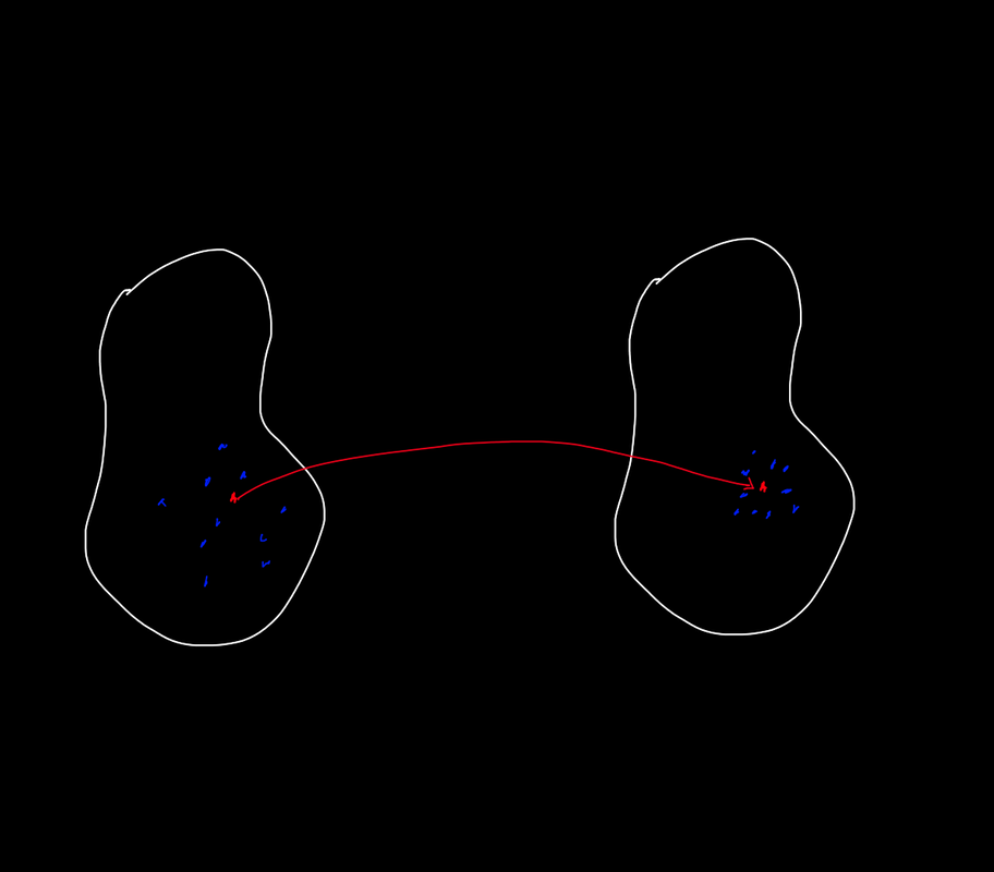 This is an example of a contraction mapping. Shown is a fixed point (in red) and some points in a neighborhood of it (in blue). Perhaps this visualization reminds you of something. Indeed, a homothety on the plane is an example (in particular, a special case) of a contraction mapping on \(\mathbb{R}^2\) to \(\mathbb{R}^2\)! How so? 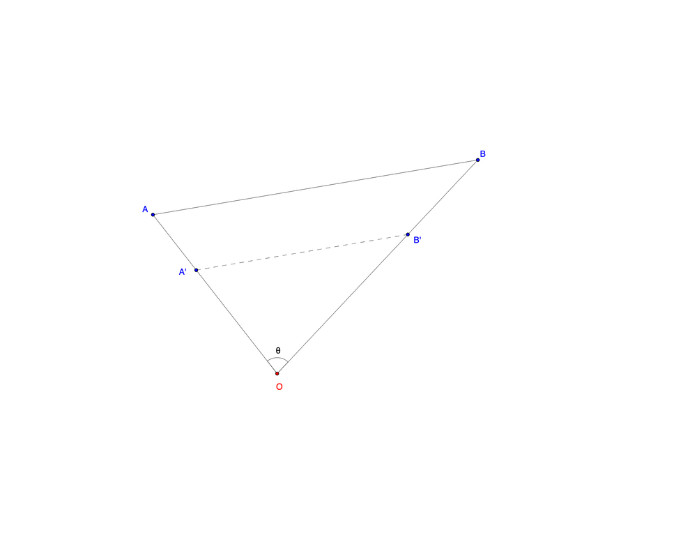 This is a homothety with center \(O\).
Consider two arbitrary points \(A\) and \(B\) in \(\mathbb{R}^2\), along with an arbitrary center \(O\). By the law of cosines, \[d(A,B)^2=d(A,O)^2+d(B,O)^2-2d(A,O)d(B,O)\cos{\theta},\] where \(\theta=\angle AOB\). Now take a homothety about \(O\) with scale factor \(0<k<1\). The operation takes every point in the plane and multiplies its distance to \(O\) by \(k\). Denote the image of \(P\) as \(h(P)\). Since homotheties preserve angles, we have again by the law of cosines, \[\begin{split} d(h(A),h(B))^2&=d(h(A),h(O))^2+d(h(B),h(O))^2-2d(h(A),h(O))d(h(B),h(O))\cos{\theta}\\ &=k^2[d(A,O)^2+d(B,O)^2-2d(A,O)d(B,O)\cos{\theta}]\\ &=k^2d(A,B)^2, \end{split}\] so \(d(h(A),h(B))=kd(A,B)\). Hence, we can choose \(c=k+\frac{1-k}{2}\) to satisfy the definition of a contraction mapping. The beautiful thing about this special case is that it makes it viscerally clear what it is we are generalizing. The contraction mapping theorem implies that there is a fixed point for our homothety. Indeed, \(O\) is a fixed point! Everything gets "squished" towards \(O\). Obviously it is no surprise that \(O\) is a fixed point – this follows trivially from the definition of a homothety (\(0\cdot k=0\)). The contraction mapping theorem is a stronger statement which essentially says that a more general "squishing" function still has "centers" that don't move. I will relegate the proof of the contraction mapping theorem to an actual PDF post, but I figured I should give a little background and context here. The proof is the one covered at UC San Diego's MATH 31BH. |
Categories
All
Archives
July 2023
|
 RSS Feed
