|
This last week in MATH 31BH, I learned of the proof of the inverse function theorem. The theorem states that if we have a function \(f\colon U\to\mathbb{R}^n\) where \(U\) is an open subset of \(\mathbb{R}^n\) and \([Df(\vec{x_0})]\) is invertible, then \(f\) is locally invertible at \(\vec{x_0}\). Honestly, this result isn't particularly interesting to me. It is too natural and intuitive. It would be a lot more interesting if the result were the opposite of what it is. After all, the total derivative is the best local affine approximation of a function. It isn't very extraordinary that a function preserves the invertibility of its approximation. However, the proof of the inverse function theorem requires what is known as the contraction mapping theorem (also called the Banach fixed-point theorem), which is a central result in analysis. This is a lot more interesting as it almost makes sense if you try to visualize it. Here is the theorem. Theorem (Contraction Mapping Theorem): Let \(f\colon\overline{U}\to\overline{U}\) be continuous. Suppose that \(\exists c\in(0,1)\) such that \[|f(\vec{x})-f(\vec{y})|<c|\vec{x}-\vec{y}|\] \(\forall\vec{x},\vec{y}\in U\). Then, \(\vec{x}\) such that \(f(\vec{x})=\vec{x}\) (a fixed point). Ah! This makes great sense. If you squish some points together, it would seem that some point must not move. Behold my great visualization. 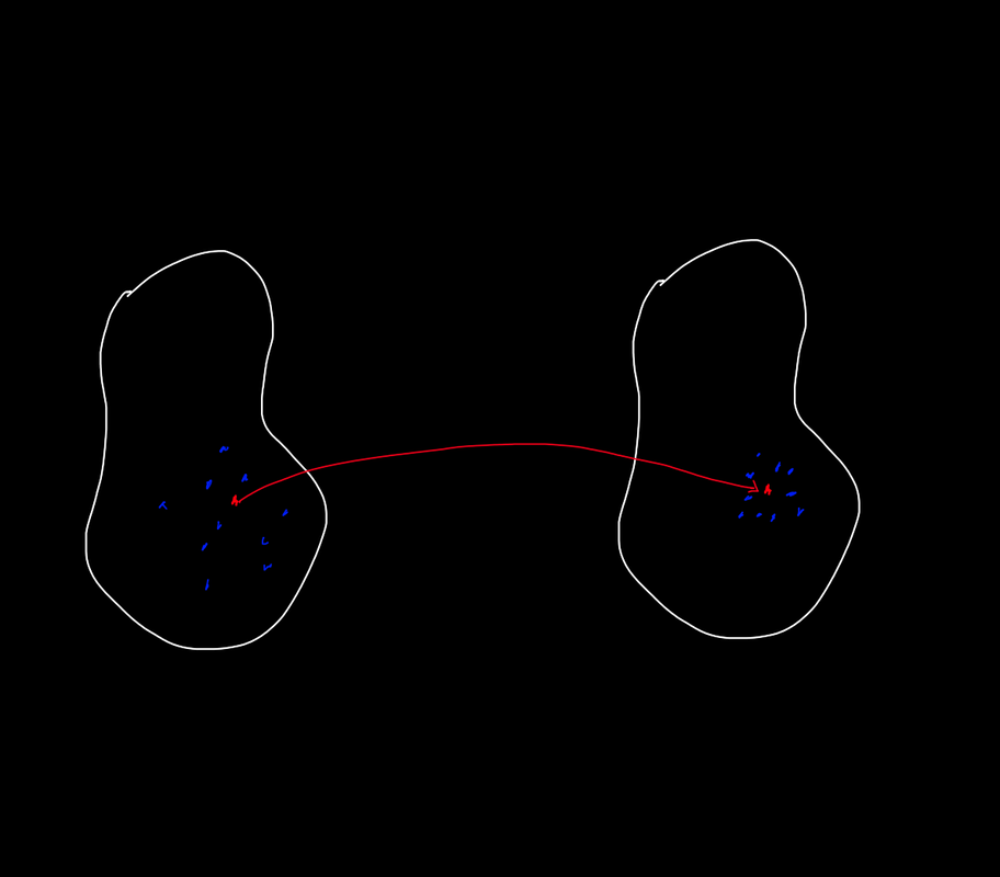 This is an example of a contraction mapping. Shown is a fixed point (in red) and some points in a neighborhood of it (in blue). Perhaps this visualization reminds you of something. Indeed, a homothety on the plane is an example (in particular, a special case) of a contraction mapping on \(\mathbb{R}^2\) to \(\mathbb{R}^2\)! How so? 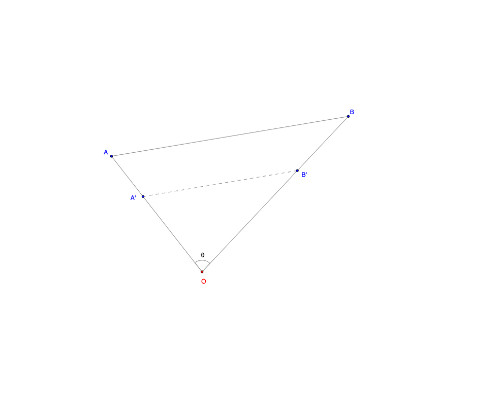 This is a homothety with center \(O\).
Consider two arbitrary points \(A\) and \(B\) in \(\mathbb{R}^2\), along with an arbitrary center \(O\). By the law of cosines, \[d(A,B)^2=d(A,O)^2+d(B,O)^2-2d(A,O)d(B,O)\cos{\theta},\] where \(\theta=\angle AOB\). Now take a homothety about \(O\) with scale factor \(0<k<1\). The operation takes every point in the plane and multiplies its distance to \(O\) by \(k\). Denote the image of \(P\) as \(h(P)\). Since homotheties preserve angles, we have again by the law of cosines, \[\begin{split} d(h(A),h(B))^2&=d(h(A),h(O))^2+d(h(B),h(O))^2-2d(h(A),h(O))d(h(B),h(O))\cos{\theta}\\ &=k^2[d(A,O)^2+d(B,O)^2-2d(A,O)d(B,O)\cos{\theta}]\\ &=k^2d(A,B)^2, \end{split}\] so \(d(h(A),h(B))=kd(A,B)\). Hence, we can choose \(c=k+\frac{1-k}{2}\) to satisfy the definition of a contraction mapping. The beautiful thing about this special case is that it makes it viscerally clear what it is we are generalizing. The contraction mapping theorem implies that there is a fixed point for our homothety. Indeed, \(O\) is a fixed point! Everything gets "squished" towards \(O\). Obviously it is no surprise that \(O\) is a fixed point – this follows trivially from the definition of a homothety (\(0\cdot k=0\)). The contraction mapping theorem is a stronger statement which essentially says that a more general "squishing" function still has "centers" that don't move. I will relegate the proof of the contraction mapping theorem to an actual PDF post, but I figured I should give a little background and context here. The proof is the one covered at UC San Diego's MATH 31BH.
0 Comments
|
Categories
All
Archives
July 2023
|
 RSS Feed
