|
Group actions are a powerful tool for establishing some very concrete results. One classic application is the classification of the finite subgroups of \(\mathrm{SO}(3)\). We will explore group actions more by establishing Burnside's lemma and Cayley's theorem. The central result in the theory of group actions is the orbit-stabilizer theorem. For a group \(G\) acting on a set \(S\), and for any fixed \(s\in S\), the orbit-stabilizer theorem establishes the existence of a bijection between the set of cosets of the stabilizer of \(s\) in \(G\) and the orbit of \(s\). Combining this with the counting formula tells us that if \(G_s\) is the stabilizer of \(s\) and \(O_s\) is the orbit of \(s\), we must have \[|G|=|G_s||O_s|\] if \(G\) is finite. This fact enables us to prove the following result. Burnside's Lemma: Let \(G\) be a finite group acting on the finite set \(S\). For each \(s\in S\) let \(S_g=\{s\in S\colon gs=s\}\). If \(N\) is the number of orbits induced by the group action, then \[|G|\cdot N=\sum_{g\in G}{|S^g|}.\] Proof: Let us label the unique orbits as \(O_{s_1},\dots,O_{s_N}\). Since the orbits partition \(S\), we have \[\begin{split} \sum_{s\in S}{\frac{1}{|O_s|}}&=\sum_{j=1}^{N}{\sum_{s\in O_{s_j}}{\frac{1}{|O_s|}}}\\ &=\sum_{j=1}^{N}{1}\\ &=N. \end{split}\] Multiplying both sides by \(|G|\) gives us \[|G|\cdot N=\sum_{s\in S}{\frac{|G|}{|O_s|}}.\] Let \(G_s\) be the stabilizer of \(s\). By the counting formula, we can rewrite the summand to obtain \[|G|\cdot N=\sum_{s\in S}{|G_s|}.\] Consider every formula of the form \(gs=s\) that is true under the group action, where \(g\in G\) and \(s\in S\). Each such formula corresponds to exactly one element in \(G_s\) (namely \(g\)) and one element in \(S^g\) (namely \(s\)). Conversely, every element in \(G_s\times \{s\}\) corresponds to exactly one formula of the aforementioned form, and similarly every element in \(S^g\times \{g\}\) corresponds to exactly one formula of the aforementioned form. So the following diagram commutes: 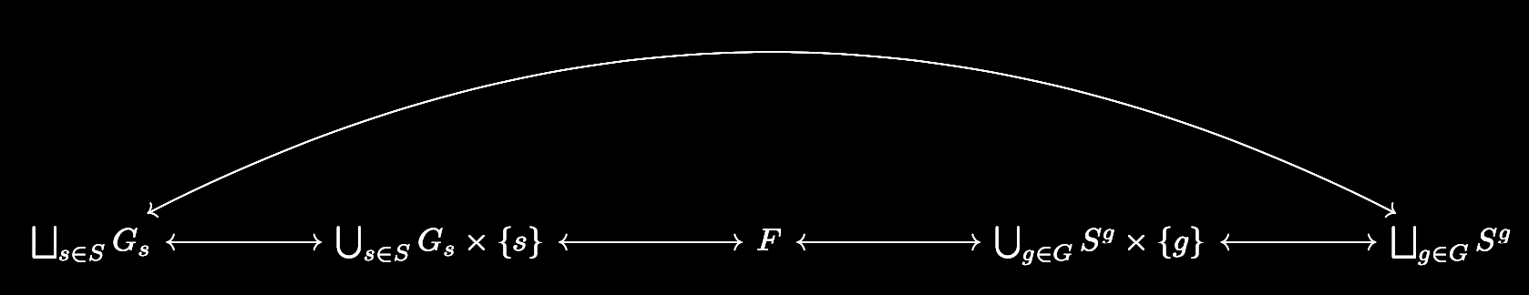 where \(F\) is the set of all formulas of the aforementioned form and all of the arrows are bijections. In particular, the bijection \(\bigsqcup_{s\in S}{G_s}\leftrightarrow\bigsqcup_{g\in G}{S^g}\) implies that
\[\sum_{s\in S}{|G_s|}=\sum_{g\in G}{|S^g|},\] and we are done. \(\square\) Burnside's lemma finds application in places where we wish to compute the number of orbits \(N\). For instance, consider the set \(S\) of \(\binom{8}{4}=70\) colorings of an octagon where four of the edges must be black and the other four must be white. Since it forms the symmetries of the octagon, the dihedral group \(D_8\) acts on this set, and we may consider orbits of this action to correspond to unique colorings. How many unique colorings are there? By Burnside's lemma, the answer is \(\frac{1}{16}\sum_{g\in D^8}{|S^g|}\). Notice by our work above, this is the same thing as \(\frac{1}{16}\sum_{s\in S}{|G^s|}\). Why do we bother using the former sum over the latter? More deeply, why did Burnside (actually, it wasn't him) care more about expressing \(N\) in terms of \(\sum_{g\in G}{|S^g|}\) rather than \(\sum_{s\in S}{|G_s|}\)? Our example hints at the answer. \(S^g\) represents the subset of colorings that remain fixed by the single symmetry \(g\). On the other hand, \(G_s\) represents the subgroup of symmetries that remain fixed by the single coloring \(s\). A little bit of thought is sufficient to see that \(S^g\) is in general a much simpler object to understand than \(G_s\). This holds in general: if the group acting on the set has a very complicated structure, it is very difficult to study the subgroup of it that fixes a single element of the set that it acts on. On the other hand, sets do not have any structure—they only have elements. By holding a group element fixed, the task becomes a matter of checking which elements in the set are fixed by that group element. This is a much easier task as it avoids the trouble of dealing with a potentially complicated group structure. In our case, this is to say that it is much easier to find the set of colorings that remain fixed under a given symmetry of the octagon than it is to find the set of symmetries that fix a given coloring of the octagon. We can push group actions even further. Let \(G\) be a group. Let \(S\) be a set, and let \(\mathrm{Perm}\ S\) denote its permutations. Note that in the category of sets, the morphisms are just functions, so \(\mathrm{Perm}\ S\) is really just the automorphism group of \(S\). In particular, it has a group structure, and there may exist a homomorphism \(\varphi\colon G\to\mathrm{Perm}\ S\). Such a homomorphism is called a permutation representation of \(G\) (with respect to \(S\)). It is not hard to see that the set of group actions of \(G\) on \(S\) has a bijective correspondence with the set of permutation representations of \(G\) with respect to \(S\). For example, let \(A\) be a group action. Then it can be checked that the map \(\varphi_A\colon G\to S_n\) which sends \(g\in G\) to the automorphism on \(S\) which is \(A\)-multiplication by \(g\) is indeed a homomorphism. Conversely, it may be checked that any permutation representation defines an action of \(G\) on \(S\). This natural correspondence gives us a natural way to identify group actions. If the permutation representation corresponding to a group action is injective, we say that the group action is faithful. Faithfulness is of course equivalent to the kernel of the corresponding permutation representation being trivial. The identity element of \(\mathrm{Perm}\ S\) is of course the identity map from \(S\) to itself. So for the kernel to be trivial, we wish left-multiplication by \(g\) to emulate the identity map on \(S\) precisely when \(g\) is the identity element of \(G\). We are now ready to prove a result that seems very deep to me at least. Cayley's Theorem: Every finite group of order \(n\) is isomorphic to a subgroup of the symmetric group \(S_n\). Proof: Let \(G\) be a finite group. Consider the group action of \(G\) on itself that maps \((g,x)\mapsto gx\). There exists a permutation representation of \(G\) with respect to itself, namely the homomorphism \(\varphi\colon G\to\mathrm{Perm}\ G\) that maps \(g\) to the automorphism on \(G\) that is left-multiplication by \(g\). Of course, the only element \(g\in G\) such that \(gx=x\) for every \(x\in G\) is the identity, so this group action is faithful. In particular, \(\varphi\) is an injective homomorphism, so \(G\) is isomorphic to \(\varphi(G)\). But of course, \(\mathrm{Perm}\ G\) is isomorphic to \(S_n\) where \(n=|G|\). \(\square\) So in an abstract sense, the symmetric groups are complicated enough that they encode every other possible finite group. This is an interesting result. However, it turns out that the idea of a group acting on itself is what really matters here, and it is that concept which is eventually used to obtain the Sylow theorems.
0 Comments
One of the greatest advantages of the Lebesgue integral over the Riemann integral is its good behavior under limits. There are three big theorems in measure theory that demonstrate this feature of the Lebesgue integral. The first of these is the monotone convergence theorem.
Monotone Convergence Theorem: If \(\{f_n\}\) is a convergent sequence in \(L^+\) such that \(f_j\leq f_{j+1}\) for all \(j\), then \(\int{\lim_{n\to\infty}{f_n}}=\lim_{n\to\infty}{\int{f_n}}\). Proof: Suppose that the measure space we are working in is \((X,\mathscr{M},\mu)\). First, note that \(\{f_n\}\) is an increasing sequence of functions, so \(\{\int{f_n}\}\) is an increasing sequence of real numbers. Thus, \(\lim_{n\to\infty}{\int{f_n}}\) exists, at least in the extended real numbers. Put \(f=\lim_{n\to\infty}{f}\). Secondly, since \(\int{f_n}\leq\int{f}\) for all \(n\), we also have that \(\lim_{n\to\infty}{\int{f_n}}\leq\int{f}\). It remains to prove the reverse inequality. Pick a simple function \(\phi\) such that \(0\leq\phi\leq f\). Let \(\alpha\in(0,1)\) be arbitrary. Define \(E_n=\{x\in X\colon f_n(x)\geq \alpha\phi(x)\}\). Since the \(f_n\) are increasing, \(f_n(x)\geq\alpha\phi(x)\) will imply \(f_m(x)\geq\alpha\phi(x)\) for all \(m\geq n\). Hence, the \(E_n\) are an increasing sequence of sets: \(E_1\subseteq E_2\subseteq \dots\). Fix \(x\in X\). The sequence \(\{f_n(x)\}\) is an increasing sequence of real numbers converging to \(f(x)\). Hence, there exists some \(N\) such that for all \(n>N\) we have that \(0\leq f(x)-f_n(x)\leq f(x)-\alpha\phi(x)\). So for all \(n>N\) we have \(f_n(x)\geq\alpha\phi(x)\) so \(x\in E_n\). In particular, \(X=\bigcup_{n=1}^{\infty}{E_n}\). By the definitions, we have \[\int{f_n}\geq\int_{E_n}{f_n}\geq\alpha\int_{E_n}{\phi}.\] Hence, \[\lim_{n\to\infty}{\int{f_n}}\geq\alpha\lim_{n\to\infty}{\int_{E_n}{\phi}}.\] Recall that for \(E\in\mathscr{M}\), the map \(E\mapsto\int_{E}{\phi}\) is itself a measure, say \(\nu\). Since the \(E_n\) are increasing, by continuity from below on the measure \(\nu\), we have that \[\lim_{n\to\infty}{\int_{E_n}{\phi}}=\int_{\bigcup_{n=1}^{\infty}{E_n}}{\phi},\] so our inequality becomes \[\lim_{n\to\infty}{\int{f_n}}\geq\alpha\int{\phi}.\] Since this holds for \(\alpha\in(0,1)\), it will hold for \(\alpha=1\). Hence, \[\lim_{n\to\infty}{\int{f_n}}\geq\int{\phi}.\] Finally, taking the supremum over all simple functions \(\phi\leq f\), we obtain the desired inequality \[\lim_{n\to\infty}{\int{f_n}}\geq\int{f}.\] \(\square\) The definition of \(\int{f}\) requires us to consider the supremum of the set of integrals of simple functions that do not exceed \(f\), but the monotone convergence theorem tells us that we may instead compute the integral as \(\int{f}=\lim_{n\to\infty}{\int{\phi_n}}\), where \(\{\phi_n\}\) is an increasing sequence of simple functions that converges to \(f\) almost everywhere. It is a standard first result in measure theory that such sequences of simple functions exist. The monotone convergence theorem allows us to interchange integrals with limits when the limit is taken on a sequence of increasing functions. But if the dream is to be able to interchange the integral with a limit for all sequences of functions, we must prepare to be disappointed. The classic pathology is the sequence of mass functions \(f_n=\chi_{(n,n+1)}\). Of course, the sequence \(\{f_n\}\) converges pointwise to the function \(f(x)=0\), but \(\int{f_n}=1\) for all \(n\), so we clearly cannot interchange the limit and the integral in this scenario. The issue here is that even though there is convergence to a nice function, there is a non-negligible mass that preserved in every function of the sequence. A related example is given by \(f_n=n\chi_{\left(0,\frac{1}{n}\right)}\). Once again, the integral of each function in the sequence is \(1\), but the function converges pointwise to \(0\). Again, the issue is that there is a non-negligible mass that is preserved in every function of the sequence. A reasonable objection may be the following. In both examples above, the convergence is pointwise but not uniform, so perhaps the limit and integral fail to be interchangeable because the convergence is not strong enough. This is also wrong: consider \(f_n=\frac{1}{n}\chi_{(0,n)}\). In this case, \(f_n\to 0\) not just pointwise, but uniformly. Nonetheless, \(\int{f_n}=1\) for every \(n\), so the limit and integral cannot be interchanged. It turns out that the relationship between the standard modes of convergence and the limiting behavior of integrals is a subtle one which I will talk about in the future. So the failures that we have demonstrated are truly an inherent limitation of the Lebesgue integral, not a weakness of the form of convergence. Nonetheless, there is something we can say when we have no condition on the sequence of functions (not even the condition that they converge to something). Fatou's Lemma: If \(\{f_n\}\) is any sequence in \(L^+\), then \[\int{\liminf{f_n}}\leq\liminf{\int{f_n}}.\] Proof: For every \(k\geq1\) and \(j\geq k\) we have that \(\inf_{n\geq k}{f_n}\leq f_j\) and thus \(\int{\inf_{n\geq k}{f_n}}\leq\int{f_j}\). This is preserved when we take the infimum of the left: \[\int{\inf_{n\geq k}{f_n}}\leq\inf_{j\geq k}{\int{f_j}}.\] For every \(k\), let \(g_k=\inf_{n\geq k}{f_n}\) and consider the sequence of functions \(\{g_k\}\). Clearly,\(g_1\leq g_2\leq\dots\). So by the monotone convergence theorem, we have that \[\int{\liminf_{n\to\infty}{f_n}}=\int{\lim_{k\to\infty}{g_k}}=\lim_{k\to\infty}{\int{g_k}}\leq\lim_{k\to\infty}{\inf_{j\geq k}{\int{f_j}}}=\liminf_{n\to\infty}{\int{f_n}}.\] \(\square\) Fatou's lemma can be used to derive another proof of the monotone convergence theorem. Second Proof (Monotone Convergence Theorem): Recall that in the first proof, it was immediate that \(\lim_{n\to\infty}{\int{f_n}}\leq\int{f}\), so it suffices to show the reverse inequality. But this is immediate by Fatou's lemma. In particular, if a limit exists, it is equal to the limit infimum, so \(f=\liminf_{n\to\infty}{f_n}\) and \(\lim_{n\to\infty}{\int{f_n}}=\liminf_{n\to\infty}{\int{f_n}}\). \(\square\) Fatou's lemma has weak hypotheses but is a weak result. Moreover, one may ask: what about sequences in \(L^1\)? So far we have only been dealing with sequences in \(L^+\). The dominated convergence theorem is the main result that we use in practice, and is arguably one of the most important results in measure theory. Dominated Convergence Theorem: Let \(\{f_n\}\) be a convergent sequence in \(L^1\) such that there exists \(g\in L^1\) with \(|f_n|\leq g\) almost everywhere for all \(n\), then \(\lim_{n\to\infty}{f_n}\in L^1\) and \(\int{\lim_{n\to\infty}{f_n}}=\lim_{n\to\infty}{\int{f_n}}\). Proof: Let \(\lim_{n\to\infty}{f_n}=f\) almost everywhere. Some standard results show that \(f\) is measurable. Since \(|f|\leq g\in L^1\), we must have that \(f\in L^1\). Suppose that the \(f_n\) are real-valued. By the hypothesis, we have that \(g+f_n\geq0\) and \(g-f_n\geq0\) almost everywhere. Now we can compute \[\begin{split} \int{g}+\int{f}&=\int{g+f}\\ &=\int{\left(g+\lim_{n\to\infty}{f_n}\right)}\\ &=\int{\liminf_{n\to\infty}{\left(g+f_n\right)}}\\ &\leq\liminf_{n\to\infty}{\int{(g+f_n)}}\\ &=\int{g}+\liminf_{n\to\infty}{\int{f_n}}, \end{split}\] where we invoke Fatou's lemma to obtain the inequality. Similarly, \[\begin{split} \int{g}-\int{f}&=\int{g-f}\\ &=\int{\left(g-\lim_{n\to\infty}{f_n}\right)}\\ &=\int{\liminf_{n\to\infty}{\left(g-f_n\right)}}\\ &\leq\liminf_{n\to\infty}{\int{(g-f_n)}}\\ &=\int{g}-\limsup_{n\to\infty}{\int{f_n}}. \end{split}\] Rearranging the two inequalities gives us \(\liminf_{n\to\infty}{\int{f_n}}\geq\int{f}\) and \(\int{f}\geq\limsup_{n\to\infty}{\int{f_n}}\). So it follows that \[\int{f}=\lim_{n\to\infty}{\int{f_n}}.\] In general, if the \(f_n\) are not real-valued, we can break it up into the positive and negative parts of its real and imaginary parts and apply the same procedure as above to arrive at the conclusion. \(\square\) The dominated convergence theorem shows up in the proofs of many other foundational theorems of measure theory, as it accepts a mild hypothesis and permits one to interchange a limit and integral in exchange, which is a very useful operation. To get some more feel for the three big convergence theorems, we will interpret them in a special case. Consider the measure space \((\mathbb{N},\mathscr{P}(\mathbb{N}),\mu)\) where \(\mu\) is the counting measure. Let \(\{f_n\}\) be an arbitrary sequence in \(L^+\) (with respect to this measure space). What does this really mean? For each \(n\), we may construct the family of simple functions \(\{\phi_m^n\}\) as follows. First, define \[\phi_1^n=f_n(1)\chi_{f_n^{-1}(f_n(1))}.\] Define, \[A_m=\mathbb{N}\setminus\bigcup_{j=1}^{m}{f_n^{-1}(f_n(k))}.\] For \(m>1\), if \(A_m=\varnothing\), set \(\phi_m^n=\phi_{m-1}^n\). Otherwise, let \(k_m\) be the minimal element of \(A_m\) and set \[\phi_m^n=\phi_{m-1}^n+f_n(k_m)\chi_{f_n^{-1}(f_n(k_m))}.\] Observe that by construction, \(\lim_{m\to\infty}{\phi_m^n}=f_n\) everywhere, and \(m\), \(\phi_1^n\leq\phi_2^n\leq\dots\leq f_n\). So by the monotone convergence theorem, \[\int{f_n}=\lim_{m\to\infty}{\int{\phi_m^n}}=\sum_{k=1}^{\infty}{f_n(k)},\] where the sum comes from the construction of \(\phi_m^n\) and the fact that \(\mu\) is the counting measure. So we may interpret \(\int{f_n}\) as simply the sum of its values. In particular, there is a correspondence between functions in \(L^+\) with respect to our measure space and sequences of numbers in \([0,\infty]\). Let \(\{S_n\}\) be a family of such sequences, where \[S_n=s_{n,1},s_{n,2}\dots\] and let \(\{f_n\}\) be the family of functions in \(L^+\) such that \(f_n(k)=s_{n,k}\). Let \(T\) be the sequence given by \[T=t_1,t_2,\dots\] where \(t_k=\liminf_{n\to\infty}{s_{n,k}}\). Corresponding to this sequence is the function \(\liminf_{n\to\infty}{f_n}\). Hence, Fatou's lemma tells us that \[\sum_{k=1}^{\infty}{\liminf_{n\to\infty}{s_{n,k}}}\leq\liminf_{n\to\infty}\sum_{k=1}^{\infty}{s_{n,k}}.\] Now, let us further insist that the sequences \(S_n\) are such that for each \(k\), \(s_{1,k}\leq s_{2,k}\leq\dots\). Of course, for each \(k\), \(\lim_{n\to\infty}{s_{n,k}}\) is guaranteed to exist due to the compactness of \([0,\infty]\). Then by the monotone convergence theorem, \[\lim_{n\to\infty}{\sum_{k=1}^{\infty}{s_{n,k}}}=\sum_{k=1}^{\infty}{\lim_{n\to\infty}{s_{n,k}}}.\] We need some extra work to interpret the dominated convergence theorem in this context. Integrals of functions \(\mathbb{N}\to\mathbb{C}\) can still be interpreted as the infinite sum of their values by splitting up the function into the positive and negative parts of its real and imaginary parts and applying our work above on \(L^+\) functions, and using the linearity of the integral. Suppose that \(\{f_n\}\) is a sequence of functions \(\mathbb{N}\to\mathbb{C}\) in \(L^1\) such that \(f_n\to f\) almost everywhere and there is a nonnegative \(g\in L^1\) such that \(g\geq|f_n|\) almost everywhere for each \(n\). Note that the functions \(|f_n|\) are in \(L^+\), and by our previous interpretation of such functions, they correspond to sequences of numbers from \([0,\infty]\). Hence, the condition \(f_n\in L^1\) is equivalent to \[\sum_{k=1}^{\infty}{|f_n(k)|}<\infty.\] Observe that in the measure space \((\mathbb{N},\mathscr{P}(\mathbb{N}),\mu)\), the only null set is the empty set. Hence, convergence almost everywhere is equivalent to convergence everywhere in this context. In particular, for each \(k\), \(f(k)=\lim_{n\to\infty}{f_n(k)}\). Moreover, notice that \(g\) is in \(L^+\), so \[\sum_{k=1}^{\infty}{|f_n(k)|}\leq\sum_{k=1}^{\infty}{g(k)}<\infty.\] So the interpretation is the following. Let \(\{S_n\}\) be a family of sequences of complex numbers \[S_n=s_{n,1},s_{n,2},\dots,\] such that for each \(k\), \(\lim_{n\to\infty}{s_{n,k}}\) exists, and there exists a sequence of nonnegative real numbers \(s_1,s_2,\dots\) with \[\sum_{k=1}^{\infty}{|s_{n,k}|}\leq\sum_{k=1}^{\infty}{s_k}<\infty,\] for each \(n\). By the dominated convergence theorem, \[\sum_{k=1}^{\infty}{\lim_{n\to\infty}{s_{n,k}}}=\lim_{n\to\infty}{\sum_{k=1}^{\infty}{s_{n,k}}},\] and moreover, \[\sum_{k=1}^{\infty}{\lim_{n\to\infty}{|s_{n,k}|}}<\infty.\] Complex differentiability is a famously strong condition, especially when it occurs in a neighborhood of every point in the domain. One longstanding question that I had was about the qualitative difference between the complex derivative and the standard Fréchet derivative from multivariable calculus.
To be precise, suppose that \(f\colon\mathbb{R}^2\to\mathbb{R}^2\) is a function given by \(f(x,y)=(u(x,y),v(x,y))\). Let \(h\colon\mathbb{C}\to\mathbb{R}^2\) be the canonical identification \(h(x+yi)=(x,y)\), and let \(g\colon\mathbb{C}\to\mathbb{C}\) be given by \(g=h^{-1}\circ f\circ h\). Observe that there is a natural correspondence between \(f\) and \(g\), and we very well could have defined \(g\) first and then \(f\) (formally, \(f\) and \(g\) are related by conjugation which is an inner automorphism). What is the relationship between the Fréchet differentiability of \(f\) and the complex differentiability of \(g\)? When both derivatives exist, what is the relationship between the Fréchet derivative \(Df\) and the complex derivative \(g'\)? First, suppose \(g\) is complex differentiable at \(z\in\mathbb{C}\). Then, \[g'(z)=\lim_{w\to0}{\frac{g(z+w)-g(z)}{w}}\] exists. Pick \(\epsilon>0\). By the above, there exists \(\delta>0\) such that \(0<|w|<\delta\) implies that \[\left|\frac{g(z+w)-g(z)}{w}-g'(z)\right|=\frac{|g(z+w)-g(z)-wg'(z)|}{|w|}<\epsilon.\] In other words, we have that \[\lim_{w\to0}{\frac{|g(z+w)-g(z)-wg'(z)|}{|w|}}=0.\] Suppose \(\alpha=\mathrm{Re}\ g'(z)\), \(\beta=\mathrm{Im}\ g'(z)\), \(x=\mathrm{Re}\ w\), and \(y=\mathrm{Im}\ w\). Now, if we define the linear operator \[A=\begin{bmatrix} \alpha & -\beta\\ \beta & \alpha \end{bmatrix},\] we have that \[wg'(z)=(x+yi)(\alpha+\beta i)=\alpha x-\beta y+(\alpha y+\beta x)i=h^{-1}\left(\begin{bmatrix} \alpha & -\beta\\ \beta & \alpha \end{bmatrix}\begin{bmatrix} x\\ y \end{bmatrix}\right)=(h^{-1}\circ A\circ h)(w).\] Observe that since \(\mathbb{C}\) and \(\mathbb{R}^2\) are isomorphic as metric spaces, distances between corresponding points are the same irrespective of which space we decide to compute them in. In particular, if \(t=h(w)\) and \(s=h(z)\), then \[\frac{|g(z+w)-g(z)-wg'(z)|}{|w|}=\frac{|(h\circ g)(z+w)-(h\circ g)(z)-h(wg'(z))|}{|h(w)|}.\] But by our work above, \(h(wg'(z))=(A\circ h)(w)\), so \[\frac{|g(z+w)-g(z)-wg'(z)|}{|w|}=\frac{|(h\circ g)(z+w)-(h\circ g)(z)-(A\circ h)(w)|}{|h(w)|}=\frac{|f(s+t)-f(s)-At|}{|t|}.\] Taking \(t\to\vec{0}\) is equivalent to taking \(w\to0\), hence \[\lim_{t\to\vec{0}}{\frac{|f(s+t)-f(s)-At|}{|t|}}=\lim_{w\to0}{\frac{|g(z+w)-g(z)-wg'(z)|}{|w|}}=0.\] So \(f\) is Fréchet differentiable at \(h(z)\), with Fréchet derivative \(A\) which has a simple relationship with \(g'(z)\). On the other hand, if we start with the assumption that \(f\) is Fréchet differentiable, it is not necessarily true that \(g\) is complex differentiable. For example, suppose \(f(x,y)=x^2+y^2\), so \(g(z)=|z|^2\). Obviously, \(f\) is Fréchet differentiable everywhere. But, suppose that \(z_0=a+bi\) is a nonzero complex number. Then, we can compute the limit \[L_1=\lim_{x\to0}{\frac{g(z+x)-g(z)}{x}},\] when \(x\) is restricted to the real numbers. Along this path, we compute \[\begin{split} L_1&=\lim_{x\to0}{\frac{(a-x)^2+b^2-a^2-b^2}{x}}\\ &=\lim_{x\to0}{\frac{x^2-2ax}{x}}\\ &=\lim_{x\to0}{x-2a}\\ &=-2a. \end{split}\] On the other hand, we can take a limit along the imaginary axis. Define, \[L_2=\lim_{y\to0}{\frac{g(z+yi)-g(z)}{yi}}.\] Then, \[\begin{split} L_2&=\lim_{y\to0}{\frac{a^2+(b-y)^2-a^2-b^2}{yi}}\\ &=\lim_{y\to0}{\frac{y^2-2by}{yi}}\\ &=\frac{1}{i}\lim_{y\to0}{y-2b}\\ &=2bi. \end{split}\] Of course, since \(z_0\neq0\), we have that \(L_1\neq L_2\), so \(g'(z_0)\) fails to exist. The complex derivative of \(g\) only exists at \(0\), where it is easily checked that \(g'(0)=0\). So the complex differentiability of \(g\) is stronger than the Fréchet differentiability of \(f\). This leads to the next natural question: what do we need in addition to the Fréchet differentiability of \(f\) to ensure the complex differentiability of \(g\)? One can easily see that our argument that the complex differentiability of \(g\) implies the Fréchet differentiability of \(f\) works in reverse. In particular, if the Fréchet derivative of \(f\) is of the form given by \(A\), then the complex derivative of \(g\) exists at the point in question where it is \(\alpha+\beta i\). We can say more if we assume continuity of the complex derivative of \(g\) and the partial derivatives of \(u\) and \(v\). Suppose \(g'\) exists in an open connected set and is continuous. One may compute the complex derivative of \(g\) in two different ways. Just as we did above, if one computes the limit along the real axis, it is immediate that \[g'(z)=\frac{\partial u}{\partial x}(h(z))+i\frac{\partial v}{\partial x}(h(z)).\] On the other hand, computing the limit along the imaginary axis gives us \[g'(z)=\frac{\partial v}{\partial y}(h(z))-i\frac{\partial u}{\partial y}(h(z)).\] Equating these two expressions for \(g'(z)\) yields the Cauchy-Riemann equations \[\frac{\partial u}{\partial x}=\frac{\partial v}{\partial y}\qquad \frac{\partial u}{\partial y}=-\frac{\partial v}{\partial x}.\] These equations are actually precisely the extra nudge that Fréchet differentiability needs to translate into complex differentiability (with the assumptions of continuity we mentioned before). To see this, suppose that \(u\) and \(v\) satisfy the Cauchy-Riemann equations in an open connected set \(G\) and that they have continuous partial derivatives. Fix \(z=x+yi\in G\). Since \(G\) is open, there exists \(r>0\) such that \(B_r(z)\subseteq G\). Let \(h=s+ti\) such that \(|h|<r\). Then, by the mean value theorem, there exists \(s_1,t_1\in\mathbb{R}\) such that \(|s_1|<|s|\), \(|t_1|<|t|\), and \[u(x+s,y+t)-u(x,y+t)=u_x(x+s_1,y+t)s\] \[u(x,y+t)-u(x,y)=u_y(x,y+t_1)t.\] Now, we may define \[\varphi(s,t)=[u(x+s,y+t)-u(x,y)]-[u_x(x,y)s+u_y(x,y)t].\] Notice that \[\begin{split} \frac{\varphi(s,t)}{s+ti}&=\frac{[u(x+s,y+t)-u(x,y)]-[u_x(x,y)s+u_y(x,y)t]}{s+ti}\\ &=\frac{[u(x+s,y+t)-u(x,y+t)]+[u(x,y+t)-u(x,y)]-[u_x(x,y)s+u_y(x,y)t]}{s+ti}\\ &=\frac{u_x(x+s_1,y+t)s+u_y(x,y+t_1)t-[u_x(x,y)s+u_y(x,y)t]}{s+ti}\\ &=\frac{s}{s+ti}[u_x(x+s_1,y+t)-u_x(x,y)]+\frac{t}{s+ti}[u_y(x,y+t_1)-u_y(x,y)] \end{split}\] Observe that \(\left|\frac{s}{s+ti}\right|,\left|\frac{t}{s+ti}\right|\leq 1\). Moreover, since \(|s_1|<|s|\) and \(|t_1|<|t|\), taking \(s,t\to0\) will force \(s_1,t_1\to0\). Hence, the last line above gives \[\lim_{s+ti\to0}{\frac{\varphi(s,t)}{s+ti}}=0.\] Similarly, one can check that \[\psi(s,t)=[v(x+s,y+t)-v(x,y)]-[v_x(x,y)s+v_y(x,y)t]\] satisfies \[\lim_{s+ti\to0}{\frac{\psi(s,t)}{s+ti}}=0.\] Now, we can compute \[\begin{split} \frac{g(z,s+ti)-g(z)}{s+ti}&=\frac{u(x+s,y+t)+iv(x+s,y+t)-u(x,y)-iv(x,y)}{s+ti}\\ &=\frac{u(x+s,y+t)-u(x,y)}{s+ti}+i\frac{v(x+s,y+t)-v(x,y)}{s+ti}\\ &=\frac{u_x(x,y)s+u_y(x,y)t+\varphi(s,t)}{s+ti}+i\frac{v_x(x,y)s+v_y(x,y)t+\psi(s,t)}{s+ti}\\ &=\frac{u_x(x,y)s+u_y(x,y)t}{s+ti}+i\frac{v_x(x,y)s+v_y(x,y)t}{s+ti}+\frac{\varphi(s,t)+i\psi(s,t)}{s+ti}\\ &=u_x(x,y)+iv_x(x,y)+\frac{\varphi(s,t)+i\psi(s,t)}{s+ti}. \end{split}\] The last line is where we finally invoke the assumption that \(u\) and \(v\) satisfy the Cauchy-Riemann equations. Taking the limit \(s+ti\to0\) and using our above results on how \(\varphi\) and \(\psi\) will behave in these limits, we obtain \[g'(z)=(u_x\circ h)(z)-i(v_x\circ h)(z).\] Since the partial derivatives of \(u\) and \(v\) are continuous and \(h\) is continuous, we conclude that \(g'\) is continuous. That is, \(g\) is continuously differentiable on \(G\). It turns out that complex differentiability in a neighborhood of every point of the domain (holomorphicity) is a strong condition that implies pretty much all the nice things that you would want. In fact, it implies that the function is infinitely complex differentiable and analytic. In the future, I will talk about these relationships, which form the core of complex analysis. There are certain theoretical preliminaries that precede the construction of most measures. One example of a measure that is more or less immediate from the definition of measures is the counting measure. It is the measure \(\mu\) on the measurable space \((X,\mathscr{P}(X))\) given by
\[\mu(E)=\sum_{x\in E}{1}.\] It is intuitive that this ought to be a measure, and it is easily checked that it is one. However, the modern construction of most other "nice" measures requires quite a bit of ground work. The first important result towards this direction is the following. Carathéodory's Theorem: Let \(\mu^*\) be an outer measure on \(X\). The collection \(\mathscr{M}\) of \(\mu^*\)-measurable subsets of \(X\) is a \(\sigma\)-algebra on \(X\), and the restriction of \(\mu^*\) to \(\mathscr{M}\) is a complete measure. As a side note, the idea of \(\mu^*\)-measurability is sometimes called the Carathéodory criterion which is that a subset \(A\) is \(\mu^*\)-measurable if for every \(B\) in the power set of \(X\), we have that \(\mu^*(B)=\mu^*(A\cap B)+\mu^*(A^c\cap B)\). Proof: It is clear by the definition of the Carathéodory criterion, and the fact that \((A^c)^c=A\), \(\mathscr{M}\) is closed under complements. It remains to show that \(\mathscr{M}\) is closed under countable unions to establish that it is a \(\sigma\)-algebra. First we show that it is closed under finite unions. Suppose \(A,B\in\mathscr{M}\). Let \(E\) be an arbitrary subset of \(X\). Then, since \(A\) is \(\mu^*\)-measurable, \[\mu^*(E)=\mu^*(E\cap A)+\mu^*(E\cap A^c).\] We can split up the first term using the \(\mu^*\)-measurability of \(B\). This gives us \[\mu^*(E)=\mu^*((E\cap A)\cap B)+\mu^*((E\cap A)\cap B^c)+\mu^*(E\cap A^c).\] Performing a similar expansion on the last term gives us \[\mu^*(E)=\mu^*(E\cap A\cap B)+\mu^*(E\cap A\cap B^c)+\mu^*(E\cap A^c\cap B)+\mu^*(E\cap A^c\cap B^c).\] In fact, the Carathéodory criterion is the natural condition on sets that allows them to be "building blocks" of other sets in the \(\mu^*\) sense. That is, for any finite collection of \(n\) \(\mu^*\)-measurable sets, the outer measure of any set can be expressed as the sum of the outer measures of intersections of the set with the \(2^n\) pieces that the collection forms. Now, observe that by Venn diagram, \(A\cup B=(A\cap B)\cup(A\cap B^c)\cup(A^c\cap B)\). It follows that \(E\cap(A\cup B)=(E\cap A\cap B)\cup(E\cap A\cap B^c)\cup(E\cap A^c\cap B)\). Subadditivity then yields \[\mu^*(E\cap(A\cup B))\leq\mu^*(E\cap A\cap B)+\mu^*(E\cap A^c\cap B)+\mu^*(E\cap A\cap B^c).\] To this, we add the De Morgan's law identity \(\mu^*(E\cap(A\cup B)^c)=\mu^*(A\cap A^c\cap B^c)\) to obtain \[\mu^*(E\cap (A\cup B))+\mu^*(E\cap(A\cup B)^c)\leq\mu^*(E).\] Of course, the reverse inequality follows immediately from subadditivity. Hence, \(\mathscr{M}\) is closed under finite unions and is at least an algebra. The outer measure is also at least finitely additive take \(A,B\in\mathscr{M}\) to be disjoint. Then, we have \[\mu^*(A\cup B)=\mu^*((A\cup B)\cap A)+\mu^*((A\cup B)\cap A^c)=\mu^*(A)+\mu^*(B).\] We need to extend these results to the countable case in order to establish the first part of the theorem. It suffices to consider a countable collections of disjoint sets from \(\mathscr{M}\), because the union of arbitrary countable collections from \(\mathscr{M}\) can be expressed as the union of a countable collection of disjoint sets from \(\mathscr{M}\) via the standard trick. So we let \(A_1,A_2,\dots\in\mathscr{M}\) be pairwise disjoint. Define \[B_n=\bigcup_{j=1}^{n}{A_j}\qquad B=\bigcup_{j=1}^{\infty}{A_j}.\] For any \(n\), since \(A_n\in\mathscr{M}\), we have that \[\mu^*(E\cap B_n)=\mu^*(E\cap B_n\cap A_n)+\mu^*(E\cap B_n\cap A_n^c).\] By definition, the first term is \(\mu^*(E\cap A_n)\) while the second term is \(\mu^*(E\cap B_{n-1})\). Repeating this inductively, we obtain that \[\mu^*(E\cap B_n)=\sum_{j=1}^{n}{\mu^*(E\cap A_j)}.\] Now, observe that \(B_n\subseteq B\), so \(B^c\subseteq B_n^c\) and \(E\cap B^c\subseteq E\cap B_n^c\). By monotonicity, we then have that \(\mu^*(E\cap B^c)\leq\mu^*(E\cap B_n^c)\). To this we add the identity above (reversed) to obtain \[\mu^*(E\cap B^c)+\sum_{j=1}^{n}{\mu^*(E\cap A_j)}\leq\mu^*(E\cap B_n^c)+\mu^*(E\cap B_n)=\mu^*(E).\] The far RHS comes from the fact that \(B_n\in\mathscr{M}\), since we have already established that \(\mathscr{M}\) is an algebra. Now, we take \(n\to\infty\) so that \[\begin{split} \mu^*(E)&\geq\mu^*(E\cap B^c)+\sum_{j=1}^{\infty}{\mu^*(E\cap A_j)}\\ &\geq\mu^*(E\cap B^c)+\mu^*\left(\bigcup_{j=1}^{\infty}{E\cap A_j}\right)\\ &=\mu^*(E\cap B^c)+\mu^*(E\cap B)\\ &\geq\mu^*(E). \end{split}\] The second line comes from countable subadditivity, the third line is by definition, and the last line comes from finite subadditivity. Note that we cannot immediately suppose that we have equality in the last line, because that would assume that \(B\in\mathscr{M}\), which is what we want to show in the first place. In any case, we have bounded \(\mu^*(E\cap B^c)+\mu^*(E\cap B)\) above and below by \(\mu^*(E)\), so in fact we do have equality in the last line. This establishes that \(\mathscr{M}\) is a \(\sigma\)-algebra. Countable additivity on \(\mathscr{M}\) comes immediately by taking \(E=B\). It remains to show that \(\mu^*|_{\mathscr{M}}\) is a complete measure. We already know that \(\mu^*\) will vanish on subsets of null sets by monotonicity. So we just need to show that subsets of null sets in \(\mathscr{M}\) are themselves in \(\mathscr{M}\). Let \(\mu^*(A)=0\). Then, by subadditivity, \(\mu^*(E)\leq\mu^*(E\cap A)+\mu^*(E\cap A^c)\), while by monotonicity, \(\mu^*(E\cap A)=0\) and \(\mu^*(E\cap A^c)\leq\mu^*(E)\), hence, \[\mu^*(E)\leq\mu^*(E\cap A^c)\leq\mu^*(E).\] Hence, \(A\) is \(\mu^*\)-measurable. In particular, if \(A'\subseteq A\) then we know that \(\mu^*(A')=0\) and by the above, \(A'\in\mathscr{M}\). We are done. \(\square\) Combining Carathéodory's theorem with the fact that premeasures on an algebra induce an outer measure, and every set in the algebra is measurable with respect to that outer measure, one can establish that a premeasure on an algebra can be extended to a measure on the generated \(\sigma\)-algebra. In fact: it is precisely the restriction of the induced outer measure to the generated \(\sigma\)-algebra. It turns out that this is the natural extension of the premeasure in the sense that the extension is unique if the premeasure is \(\sigma\)-finite, and in the general case, any other measure that extends the premeasure will be equal to the extension defined above on sets with finite measure. The construction of the Lebesgue measure thus proceeds by defining the natural premeasure on the set of half-open half-closed intervals on the real line, checking that this indeed a premeasure on an algebra, and then invoking the above result which tells us that it extends to a measure on the Borel \(\sigma\)-algebra of \(\mathbb{R}\). The completion of this measure is what we call Lebesgue measure. Taking the completion explodes the domain of the measure to a pretty large \(\sigma\)-algebra. In fact, the \(\sigma\)-algebra of Lebesgue measurable sets is so large that it has been shown that it is impossible to show that there is a Lebesgue nonmeasurable set without the axiom of choice. See here. |
Categories
All
Archives
July 2023
|
 RSS Feed
