|
I have finished my undergraduate degree at UCSD. I will begin my PhD at UNC Chapel Hill next month. My interests are roughly in geometry, topology, and mathematical physics. My last year at UCSD was crucial in shaping these interests. At UNC, I am tentatively planning on working with Justin Sawon. Overall, I am glad that I was able to learn math for the last four years at UCSD and I look forward to continuing the journey at UNC.
As for the rest of this summer, I plan on reviewing some stuff that I've learned in the past few years to be relatively prepared for some of the comprehensive exams. Time-permitting, I will write up some important results here.
0 Comments
Clearly the function \(f(z)=e^z\) is an entire function that satisfies \(f(\log{n})=n\) for every \(n\in\mathbb{N}\). Are there any other such entire functions?
The answer is no if we insist that \(f\) does not grow "too quickly". We can show this by studying the relationship between the growth of an entire function and the distribution of its zeros. The fundamental result in this theory is Jensen's formula. Theorem (Jensen's formula): Let \(f\colon G\to\mathbb{C}\) be holomorphic with \(\overline{B_r(0)}\subseteq G\). Let \(a_1,\dots,a_n\) be zeros of \(f\) in \(B_r(0)\) and suppose \(f(0)\neq0\). Then, \[\log{|f(0)|}+\sum_{k=1}^{n}{\log{\frac{r}{|a_k|}}}=\frac{1}{2\pi}\int_{0}^{2\pi}{\log{|f(re^{it})|}\ \mathrm{d}t}.\] Jensen's formula tells us that the distribution of the zeros of an entire function is controlled by the growth of the function in the following sense. Corollary: Let \(f\colon\mathbb{C}\to\mathbb{C}\) be an entire function with \(f(0)=1\). For ever \(r>0\), let \(N(r)\) denote the number of zeros of \(f\) in the ball \(B_r(0)\) and let \(M(r):=\sup_{z\in B_r(0)}{|f(z)|}\). Then, for every \(r>0\), \[N(r)\log{2}\leq\log{M(2r)}.\] Proof: Pick \(r>0\). Let \(a_1,\dots,a_n\) be the roots of \(f\) in \(B_{2r}(0)\). Observe that \(\log{\left|\frac{2r}{a_k}\right|}>0\) for each \(k\) by construction. Hence, by Jensen's formula, \[\log{M(2r)}\geq\frac{1}{2\pi}\int_{0}^{2\pi}{\log{|f(2re^{it})|\ \mathrm{d}t}}=\log{|f(0)|}+\sum_{k=1}^{n}{\log{\left|\frac{2r}{a_k}\right|}}=\sum_{k=1}^{n}{\log{\left|\frac{2r}{a_k}\right|}}.\] We can break up the sum on the right hand side by considering the indices \(k\) for which \(|a_k|<r\) and the indices \(k\) for which \(r\leq|a_k|<2r\). This gives us \[\sum_{k=1}^{n}{\log{\left|\frac{2r}{a_k}\right|}}=\sum_{|a_k|<r}{\log{\left|\frac{2r}{a_k}\right|}}+\sum_{r\leq|a_k|<2r}{\log{\left|\frac{2r}{a_k}\right|}}\geq \sum_{|a_k|<r}{\log{\left|\frac{2r}{a_k}\right|}}\geq N(r)\log{2},\] with the inequalities coming from the fact that the terms in the first sum are at least \(\log{2}\) and the terms in the second sum are positive. \(\square\) This corollary leads to another way in which the growth of an entire function controls the distribution of the zeros. Let \(f\) be an entire function. Suppose \(f\) has the nonzero roots \(\{a_n\}_{n\in S}\), where \(S\) is finite or countable. The critical exponent of \(f\), denoted \(\alpha\), is defined to be \[\alpha:=\inf{\left\{t>0\colon\sum_{n\in S}{\frac{1}{|a_n|^t}}<\infty\right\}}.\] Clearly, \(\alpha\) quantifies the distribution of the zeros of \(f\) by measuring how quickly the roots of \(f\) grow: the larger \(\alpha\) is, the slower the roots of \(f\) must grow. Notice that it is very simple to see that if \(S\) is countable, then for any \(\epsilon>0\), we have \(\sum_{n\in S}{\frac{1}{|a_n|^{\alpha+\epsilon}}}<\sum_{n\in S}{\frac{1}{|a_n|^{\alpha-\epsilon}}}=\infty\). Hence, \(\alpha\) is another way to quantify the rate of decay of the terms of a series. While the behavior of the series is easy to understand when we take powers above and below \(\alpha\), it is unclear what actually happens when the power is exactly \(\alpha\). In fact, the series may either converge or diverge when we take the power to be exactly \(\alpha\). This is another sense in which the barrier between convergent and divergent series is fuzzy. Now, suppose \(f\) is an arbitrary entire function. We define the order of \(f\), denoted \(\lambda\), to be \[\lambda:=\limsup_{r\to\infty}{\frac{\log{\log{M(r)}}}{\log{r}}}.\] Clearly, \(\lambda\) is a measure of how quickly \(f\) grows. In particular, \(\lambda\) detects "exponentially polynomial" growth. That is, the order of the entire function \(\exp{z^d}\) is \(d\). The order of any polynomial is simply zero. It is fairly straightforward to show that order of a sum or product of entire functions is at most the maximal order of the addends or factors, respectively. There is a relationship between the critical exponent and the order of an entire function. This result is morally identical to our corollary: the distribution of the zeros of an entire function is controlled by the growth of the function. Proposition: Let \(f\) be an entire function with critical exponent \(\alpha\) and order \(\lambda\). Then, \(\alpha\leq\lambda\). Proof: It is clear that the order and critical exponent of an entire function is invariant under multiplication of the function by a nonzero constant, so we may assume without loss of generality that \(f(0)=1\). First, note that when \(f\) has finitely many zeros, we have \(\alpha=0\) and the conclusion is immediate. So it suffices to assume that \(f\) has countably many zeros. Suppose that the zeros of \(f\) are \(a_1,a_2,\dots\) where \(|a_1|\leq|a_2|\leq\dots\). Note that \(|a_n|\to\infty\) since otherwise \(f\) must be the constant zero function which contradicts our assumption that \(f\) has countably many roots. Then by the corollary, for every \(n\in\mathbb{N}\) we have \[n-1\leq N(|a_n|)\leq \frac{\log{M(2|a_n|)}}{\log{2}}.\] Pick \(\epsilon>0\). By the definition of order, there exists \(R\) so large that \(\log{M(r)}\leq r^{\lambda+\frac{\epsilon}{2}}\) for all \(r>R\). Since \(|a_n|\to\infty\), we have that there exists \(N\) so that for every \(n>N\) we have \[n-1\leq N(|a_n|)\leq \frac{\log{M(2|a_n|)}}{\log{2}}\leq\frac{(2|a_n|)^{\lambda+\frac{\epsilon}{2}}}{\log{2}}.\] Rearranging this inequality we obtain \[\frac{1}{|a_n|}\leq \frac{2}{[(n-1)\log{2}]^{\frac{1}{\lambda+\frac{\epsilon}{2}}}}.\] Therefore, \[\frac{1}{|a_n|^{\lambda+\epsilon}}\leq\frac{2^{\lambda+\epsilon}}{[(n-1)\log{2}]^{\frac{\lambda+\epsilon}{\lambda+\frac{\epsilon}{2}}}}.\] Since \(\frac{\lambda+\epsilon}{\lambda+\frac{\epsilon}{2}}>1\), we have that \[\sum_{n=N+1}^{\infty}{\frac{1}{|a_n|^{\lambda+\epsilon}}}\leq\sum_{n=N+1}^{\infty}{\frac{2^{\lambda+\epsilon}}{[(n-1)\log{2}]^{\frac{\lambda+\epsilon}{\lambda+\frac{\epsilon}{2}}}}}<\infty.\] Therefore, \(\sum_{n=1}^{\infty}{\frac{1}{|a_n|^{\lambda+\epsilon}}}<\infty\) so that \(\lambda+\epsilon\geq\alpha\). Since \(\epsilon\) was arbitrary, the conclusion follows. \(\square\) Notice that in our proof above, we used the fact that if the \(a_n\) were not unbounded, \(f\) must be the constant zero function. This essentially due to the Bolzano-Weierstrass theorem, which would guarantee that there the zeros of \(f\) have a limit point, from which it follows by the identity theorem that \(f\) is the constant zero function. This subtle point makes a reappearance in our main result, which we are now able to state. Theorem: Let \(f\) and \(g\) be entire functions with order at most \(\delta<\infty\). Suppose that \(\{a_n\}_{n\in\mathbb{N}}\) is a sequence of nonzero complex numbers such that \(f(a_n)=g(a_n)\) for every \(n\in\mathbb{N}\) and \[\sum_{n=1}^{\infty}{\frac{1}{|a_n|^{1+\delta}}}<\infty.\] Then, \(f=g\). Proof: Consider the entire function \(F=f-g\). Let \(0\) be a root of \(F\) with multiplicity \(m\). Then we can write \(F=z^mG\) for some entire function \(G\) where \(G(0)\neq0\) but \(G(a_n)=0\) for every \(n\). Let \(\lambda\) be the order of \(G\). We know that \(\lambda\leq\delta\) since the order of a sum is at most the maximal order of the addends. By the condition given on \(\{a_n\}_{n\in\mathbb{N}}\), we have \(\lambda+1\leq\delta+1\leq\alpha\) where \(\alpha\) is the critical exponent of \(G\). But by the previous proposition, we also have \(\alpha\leq\lambda\), hence we have \(\lambda+1\leq\lambda\), contradicting our assumption that \(\delta\) is finite. So where is the mistake? The error is in assuming that the critical exponent of \(G\) is well-defined to begin with. Recall that the definition of the critical exponent requires the entire function to have at most countably many roots. Hence, \(G\) must have have uncountably many roots. Now it is simple to show that \(G\) must be the constant zero function. We may reason as follows. Since \(\mathbb{C}\) is \(\sigma\)-compact, we can let \(\{S_n\}_{n\in\mathbb{N}}\) be a countable collection of compact subsets of \(\mathbb{C}\) such that \(\mathbb{C}=\bigcup_{n\in\mathbb{N}}{S_n}\) (one can choose, for example, closed unit squares). Let \(Z\subseteq\mathbb{C}\) be the zero set of \(G\). Suppose \(Z\cap S_n\) is finite for every \(n\in\mathbb{N}\). Then \(Z=\bigcup_{n\in\mathbb{N}}{(Z\cap S_n)}\) is countable as a countable union of finite sets, which contradicts our observation that \(Z\) is uncountable. Hence, there exists \(N\in\mathbb{N}\) such that \(Z\cap S_N\) is infinite. But since \(S_N\) is compact, it is sequentially compact, and thus \(Z\cap S_N\) has a limit point in \(S_N\). In particular, \(Z\) has a limit point so \(F\) is identically zero. \(\square\) This is a great example of why it is very important to check the hypotheses of not just theorems, propositions, and lemmas, but also definitions! The theorem essentially tells us the following. Suppose \(f\) is an entire function with order \(\lambda\) and zeros \(\{a_n\}_{n\in\mathbb{N}}\). If \(f\) grows too slowly (that is, \(\lambda\) is small) and the zeros of \(f\) do not grow very quickly (that is, \(\frac{1}{|a_n|}\) does not decay rapidly), then \(f\) is the constant zero function. We can use this idea to show that if \(g(z)=e^z\), and \(f\) is an entire function of finite order such that \(f(\log{n})=n\) for all \(n\in\mathbb{N}\), the entire function \(f-g\) is the constant zero function. In essence, we will show that if \(f\) does not grow too quickly, the roots \(\log{n}\) grow so slowly that the assumption that \(f\) is entire forces \(f(z)-e^z\) to be identically zero. Let \(g(z)=e^z\). Suppose \(f\) is an entire function of finite order such that \(f(\log{n})=n\) for all \(n\in\mathbb{N}\). \(g\) is of order \(1\) and agrees with \(f\) on \(\{\log{n}\}_{n\in\mathbb{N}}\). Let \(\lambda_f\) be the order of \(f\) and \(\delta=\max{(1,\lambda_f)}\). Notice that the orders of \(f\) and \(g\) are at most \(\delta<\infty\). Observe that if we apply L'hôpital's rule \(\left\lfloor 1+\delta\right\rfloor\) times, we obtain that \[\lim_{x\to\infty}{\frac{x}{(\log{x})^{1+\delta}}}=\lim_{x\to\infty}{\frac{x}{\left\lfloor 1+\delta\right\rfloor!(\log{x})^{\{\delta\}}}}\geq\frac{1}{\left\lfloor 1+\delta\right\rfloor!}\lim_{x\to\infty}{\frac{x}{\log{x}}}=\infty,\] where \(\{\delta\}\) is the fractional part of \(\delta\) and the last equality follows from one more application of L'hôpital's rule. So \(\lim_{x\to\infty}{\frac{x}{(\log{x})^{1+\delta}}}=\infty\). This means there exists some \(N\in\mathbb{N}\) so that for all \(n>N\), we have \(n>(\log{n})^{1+\delta}\) so that \(\frac{1}{n}<\frac{1}{(\log{n})^{1+\delta}}\). Since the harmonic series \(\sum_{n=1}^{\infty}{\frac{1}{n}}\) diverges, we note that by direct comparison, \[\sum_{n=2}^{\infty}{\frac{1}{|\log{n}|^{1+\delta}}}=\infty.\] Now by the previous theorem, it must be true that \(f=g\). So there is only one function \(f\) that can exist as described, and it is \(f(z)=e^z\). Note that the assumption that \(f\) has finite order is crucial. Often, in these types of arguments, one really needs some control over the growth of the entire function being studied. I am not sure if much can be said if we remove the requirement that \(f\) must have finite order. This theory can be pushed farther. The growth of the zeros of an entire function can be quantified in way distinct from the critical exponent. The quantity that does this is known as the genus of the entire function, and it is somewhat related to the critical exponent. If we denote the genus of an entire function as \(h\) and the order of the function as \(\lambda\), then it is true that \(h\leq\lambda\leq h+1\). This is a pretty strong relationship: it gives us a very good understanding of the growth of an entire function given the growth of its zeros. This result can be used to prove weak versions of the Picard theorems, which I think are some of the most interesting results in complex analysis. In high school calculus, one is often inundated with various series convergence tests. It is often a headache to determine which convergence test to use on a particular series. None of the high school convergence tests work on every series. For example,
The answer is no. A short and clever argument shows that an algorithm that can determine if any sequence (or equivalently, series) converges would be capable of solving the halting problem, and thus no such algorithm can exist. This result may be disappointing to high school math students. It also suggests that any notion of a "barrier" between the convergent series and the divergent series would be fuzzy at best. There are many ways to define what such a threshold could be. Intuitively, we would like to say that the threshold is some "critical rate of decay" on the terms of series (modulo trivial modifications to the series) such that a series converges if and only if the rate of decay of the terms of that series is at least the critical rate of decay. There are several different ways of making this precise. We will discuss the following way. Definition: Let \(\{a_n\}_{n\in\mathbb{N}}\) be a sequence of positive numbers. The series \(\sum_{n=1}^{\infty}{a_n}\) is said to be a threshold series (and the sequence \(\{a_n\}_{n\in\mathbb{N}}\) is a threshold sequence) if \(\sum_{n=1}^{\infty}{a_n|c_n|}<\infty\) if and only if the sequence \(\{c_n\}_{n\in\mathbb{N}}\) is bounded. Indeed, this notion of a threshold series captures what we intuitively want. Of course, modifying the terms of any series by any collection of bounded coefficients will not change the convergence of the series. Our notion of threshold series thus includes all such modifications (this is what we meant by quantifying a rate of decay of the terms of a series modulo trivial modifications). The main point is that modification by an unbounded collection of coefficients will always tip the threshold series over the edge into the realm of divergent series—no matter how slowly our coefficients grow. Thus, a threshold series is a series that exhibits a "critical rate of decay" in its terms. It turns out that our hunch that the barrier between convergent and divergent series is fuzzy is correct in the sense that threshold series do not exist. To prove this result, we will need the following lemma. Lemma: Let \(X\) and \(Y\) be topological spaces and let \(\Omega\) be a dense subset of \(Y\). If \(\varphi\colon X\to Y\) is an open map, then \(\varphi^{-1}(\Omega)\) is dense in \(X\). Proof: Pick \(x\in X\) and an open neighborhood \(U\) of \(x\). Since \(\varphi\) is an open map and \(U\) is nonempty, \(\varphi(U)\) is an open subset of \(Y\). Since \(\Omega\) is dense, there exists \(y\in\varphi(U)\cap\Omega\). In particular, since \(y\in\varphi(U)\), there exists \(x'\in U\) such that \(\varphi(x')=y\in\Omega\). Hence, \(x'\in\varphi^{-1}(\Omega)\), so \(U\cap\varphi^{-1}(\Omega)\) is nonempty. \(\square\) Now we may proceed with our main argument. We will reason by contradiction. Suppose that there exists a threshold sequence \(\{a_n\}_{n\in\mathbb{N}}\). Let \(B(\mathbb{N})\) be the space of bounded functions on \(\mathbb{N}\). We can interpret \(B(\mathbb{N})\) as a Banach space with the uniform norm (i.e. the supremum norm). Let \(\mu\) be the counting measure on \(\mathbb{N}\) so that \(L^1(\mu)\) is precisely the collection of absolutely convergent sequences. Define the map \(T\colon B(\mathbb{N})\to L^1(\mu)\) given by \((Tf)(n)=a_nf(n)\) for every \(n\in\mathbb{N}\) and \(f\in B(\mathbb{N})\). Note that the image of \(T\) is a subset of \(L^1(\mu)\) and so \(L^1(\mu)\) is a valid codomain because \(\{a_n\}_{n\in\mathbb{N}}\) is a threshold sequence. It is trivial to check that \(T\) is a surjective linear map between Banach spaces. Suppose that we have a sequence of functions \(\{g_n\}_{n\in\mathbb{N}}\subseteq B(\mathbb{N})\) such that \(g_n\to g\) and \(Tg_n\to h\) where the convergence occurs with respect to the norms of the relevant Banach spaces. Pick \(\epsilon>0\) and fix \(k\in\mathbb{N}\). Since \(g_n\to g\) in uniform norm, we have that \(g\) is the pointwise limit of the \(g_n\). In particular, we may pick \(N_1\) so large that for all \(n>N_1\) we have \(|g_n(k)-g(k)|<\frac{\epsilon}{2a_k}\). Since \(Tg_n\to h\) in the \(L^1\) norm, we pick \(N_2\) so large that for all \(n>N_2\) we have \[|a_kg_n(k)-h(k)|\leq\sum_{j=1}^{\infty}{|a_jg_n(j)-h(j)|}=\sum_{j=1}^{\infty}{|Tg_n(j)-h(j)|}=\|Tg_n-h\|_1<\frac{\epsilon}{2}.\] Now, for \(n>\max{(N_1,N_2)}\), we have \[\begin{split} |(Tg)(k)-h(k)|&=|a_kg(k)-h(k)|\\ &=|a_kg(k)-a_kg_n(k)+a_kg_n(k)-h(k)|\\ &\leq|a_kg(k)-a_kg_n(k)|+|a_kg_n(k)-h(k)|\\ &<\frac{\epsilon}{2}+\frac{\epsilon}{2}=\epsilon. \end{split}\] Since \(\epsilon\) is arbitrary, we have that \((Tg)(k)=h(k)\). Thus, \(Tg=h\). We have showed that \(T\) is a closed linear map, hence \(T\) is continuous by the closed graph theorem. Now since \(T\) is a surjective continuous linear map, \(T\) is open by the open mapping theorem. Let us define \[S=\left\{f\in B(\mathbb{N}): \left|f^{-1}(\mathbb{R}\setminus\{0\})\right|<\infty\right\}.\] It is clear that \(T^{-1}(S)=S\). Notice that for any \(f\in S\), if \(\chi_{\mathbb{N}}\in B(\mathbb{N})\) is the constant indicator function, \[\sup_{n\in\mathbb{N}}{|\chi_{\mathbb{N}}(n)-f(n)|}\geq\sup_{n\in f^{-1}(\{0\})}{|\chi_{\mathbb{N}}(n)-f(n)|}=1.\] Hence, \(S\) is not dense in \(B(\mathbb{N})\). Now pick \(\epsilon>0\) and \(f\in L^1(\mu)\). By definition, \(\sum_{n=1}^{\infty}{|f(n)|}<\infty\), so we may pick \(N\) so large that for \(m\geq N\) we have \(\sum_{n=m}^{\infty}{|f(n)|}<\epsilon\). Define the function \(g\) by \[g(n)=\begin{cases} f(n) & n<N\\ 0 & n\geq N. \end{cases}\] Note that \(g\in S\) by construction. Moreover, \[\|f-g\|_1=\sum_{n=1}^{\infty}{|f(n)-g(n)|}=\sum_{n=N}^{\infty}{|f(n)|}<\epsilon.\] This means that \(S\) is dense in \(L^1(\mu)\). So \(S\) is dense in \(L^1(\mu)\) but not \(B(\mathbb{N})\) and \(T\colon B(\mathbb{N})\to L^1(\mu)\) is an open map with \(T^{-1}(S)=S\). This contradicts the lemma, completing the argument. This is one of my favorite problems because it provides some insight to something I've always thought about when I was younger (the "barrier" between convergent and divergent series) using some comparatively abstract techniques from functional analysis. A lot was swept under the rug via the open mapping and closed graph theorems. I find it fascinating that these abstract results can tell us something that I find relatively tangible about series. The problem of measuring how quickly the terms of a series decay isn't just one from my big bag of problems that I find interesting. It is in fact well-studied in complex analysis, where many results are known regarding how quickly the zeros of an entire function grow. Allegedly, this has significant ramifications in analytic number theory. At some point in the future, I will talk about the critical exponent and the order of an entire function and the relationship between the growth of an entire function and the distribution of its zeros. One of my favorite ideas in all of mathematics is to study the topology of a space by studying functions on the space. This is the underlying idea of Morse theory, which I hope to learn more about. A huge set of examples of this idea that I am more familiar with comes from complex analysis.
One may observe that in the examples that I have given, the functions we are studying to probe the topology possess some non-topological properties. For instance, holomorphic functions famously have some extremely strong properties most of which are not topological in nature at all. The same goes for harmonic functions, which share many properties with holomorphic functions. In general, differentiability is not a property of a function that interacts much at all with the domain topology. So it is natural to wonder if we can study the topology of a space by studying functions that obey no assumption other than the assumption that they interact somehow with the topology. It also seems reasonable that the topology should be uniquely determined by such functions. More precisely, let \(X\) be a topological space and let \(C(X)\) be the ring of real-valued continuous functions on \(X\). Question: Can one recover the topology on \(X\) given \(C(X)\)? In this blog post, we will show that the answer is in the affirmative. We will focus on the following special case: fix \(X\) to be a compact Hausdorff topological space. Consider the spectrum of the ring, \(C(X)\), which we denote \(\text{Spec }C(X)\). We can interpret the spectrum as a topological space by giving it the Zariski topology. Let \(\mathscr{M}\) be the set of maximal ideals of \(C(X)\). Since every maximal ideal is prime, \(\mathscr{M}\subseteq\text{Spec }C(X)\) and we can endow \(\mathscr{M}\) with the subspace topology. We sometimes refer to \(\mathscr{M}\) as the maximal spectrum of \(C(X)\). The incredible fact which we will prove is that \(X\) is homeomorphic to \(\mathscr{M}\). For every \(x\in X\) define \(I_x=\left\{f\in C(X)\colon f(x)=0\right\}\). Clearly, \(I_x\) is an ideal of \(C(X)\). What is less clear is that \(I_x\) is always a maximal ideal. We will show this in two different ways. In the first method, we will show that any ideal properly containing \(I_x\) is the full ring \(C(X)\). Fix \(x\in X\) and pick \(g\in C(X)\setminus I_x\). Since \(X\) is Hausdorff, \(\{x\}\) is closed, and since \(g\) is continuous, \(g^{-1}(\{0\})\) is closed (and disjoint with \(\{x\}\) since \(g\notin I_x\)). Recall that every compact Hausdorff space is normal (\(T_4\)), so by Urysohn's lemma, there exists a continuous function \(f\colon X\to\mathbb{R}\) such that \(f(x)=0\) but \(f(y)=1\) for all \(y\in g^{-1}(\{0\})\). Notice that \(f\in I_x\). Moreover, \(f\) and \(g\) have no common zeros by construction. Therefore, \(f^2+g^2\in\langle f,g\rangle\) is always positive, so the multiplicative inverse \(\frac{1}{f^2+g^2}\) exists in \(C(X)\). Since ideals are closed under multiplication from any element, \(\chi_X=(f^2+g^2)\cdot\frac{1}{f^2+g^2}\in\langle f,g\rangle\). So the ideal \(\langle f,g\rangle\) contains the identity element of the ring and thus \[C(X)=\langle f,g\rangle\subseteq\langle I_x,g\rangle\subseteq C(X).\] Hence, \(I_x\) is a maximal ideal as claimed. We have established that \(\{I_x\}_{x\in X}\subseteq\mathscr{M}\). It turns out that this is method is quite clumsy. A quicker way to establish that \(I_x\) is maximal is to notice that it is the kernel of the evaluation homomorphism \(C(X)\to\mathbb{R}\) that maps \(f\mapsto f(x)\). Since the homomorphism is clearly surjective, the first isomorphism theorem tells us that \(C(X)/I_x\cong\mathbb{R}\), which is a field. This immediately tells us that \(I_x\) is maximal. Hence, Urysohn's lemma is not (yet) required. The fact that \(\{I_x\}_{x\in X}\subseteq\mathscr{M}\) is purely algebraic. We want to establish the reverse inclusion as well. This is tantamount to showing that every maximal ideal of \(C(X)\) is of the form \(I_x\) for an appropriate choice of \(x\in X\). Let us study a "rogue" maximal ideal \(I\) that is not of the form \(I_x\) for any \(x\in X\). Since \(I\) is maximal and \(I_x\) is maximal for every \(x\in X\), the containment \(I\subseteq I_x\) would immediately imply \(I=I_x\). Hence, \(I\) is not contained in any ideal of the form \(I_x\). This means that for each \(x\in X\), there exists \(f_x\in I\) such that \(f_x(x)\neq0\). For each \(x\in X\), by the continuity of each \(f_x\) and the fact that \(f_x(x)\neq0\), there exists an open neighborhood \(U_x\) of \(x\) such that \(0\notin f_x(U_x)\). This gives us an open cover \(\{U_x\}_{x\in X}\) (notice that to form this open cover, we are invoking the axiom of choice). By compactness, we may extract a finite subcover \(\left\{U_{x_j}\right\}_{j=1}^{n}\). By construction, for each \(x\in X\), there exists at least one \(1\leq j\leq n\) such that \(f_{x_j}(x)\neq0\). So the functions \(f_{x_1},\dots,f_{x_n}\) have no common zero. This means that the function \(f_{x_1}^2+\dots+f_{x_n}^2\) is always positive and so \(\frac{1}{f_{x_1}^2+\dots+f_{x_n}^2}\) is a well-defined continuous function on \(X\). Since \(f_{x_1}^2+\dots+f_{x_n}^2\in I\), we have that \(\chi_X=(f_{x_1}^2+\dots+f_{x_n}^2)\cdot\frac{1}{f_{x_1}^2+\dots+f_{x_n}^2}\in I\). This is a contradiction: no maximal ideal is the unit ideal. Hence, no "rogue" maximal ideals exist. This establishes that \(\mathscr{M}=\{I_x\}_{x\in X}\). Notice the paragraph above uses the same sum of squares trick that we used when we clumsily showed that \(\{I_x\}_{x\in X}\subseteq\mathscr{M}\). In particular, we are using the general fact that the ideal generated by any finite collection of functions in \(C(X)\) that share no common zero is the unit ideal. This is what we have essentially proven in the previous paragraph. Now consider the well-defined map \(\varphi\colon X\to\mathscr{M}\) defined by \(\varphi(x)=I_x\). The above establishes that this map is a surjection. A more subtle point is injectivity. This is where we truly need Urysohn's lemma. Pick \(x,y\in X\) to be distinct points. Since compact Hausdorff spaces are normal, and \(\{x\}\) and \(\{y\}\) are disjoint closed sets, by Urysohn's lemma there exists \(f\in C(X)\) such that \(f(x)=0\) and \(f(y)=1\neq0\). This shows that \(I_x\neq I_y\), which establishes that \(\varphi\) is an injection and thus a bijection. We will establish that \(\varphi\) is in fact a homeomorphism. To do this, we will construct a basis for the topology of \(X\) and for the topology of \(\mathscr{M}\), and show that \(\varphi\) induces a bijection between those bases. For each \(f\in C(X)\), define \[U_f=f^{-1}\left(\mathbb{R}\setminus\{0\}\right),\qquad \tilde{U}_f=\left\{I\in\mathscr{M}\colon f\notin I\right\}.\] We claim that \(\{U_f\}_{f\in C(X)}\) and \(\{\tilde{U}_f\}_{f\in C(X)}\) form bases for the topologies on \(X\) and \(\mathscr{M}\), respectively. To check this, we will use the following standard result from point-set topology. A collection of open subsets \(\mathscr{E}\) of a topological space is a basis for the topology if and only if
We continue to establish the claim that \(\{\tilde{U}_f\}_{f\in C(X)}\) forms a basis for the topology on \(\mathscr{M}\). This is easy with a little knowledge of the Zariski topology on the spectrum of a ring. Define \[X_f=\left\{I\in\text{Spec }C(X)\colon f\notin I\right\}.\] It is a standard fact that \(\{X_f\}_{f\in C(X)}\) forms a basis for the Zariski topology. It is also clear that since \(\tilde{U}_f=\mathscr{M}\cap X_f\) for every \(f\in C(X)\), we have that \(\{\tilde{U}_f\}_{f\in C(X)}\) forms a basis for the subspace topology on \(\mathscr{M}\). Finally, we will establish that for every \(f\in C(X)\), we have \(\varphi(U_f)=\tilde{U}_f\). But this can be done in a single line. \[\varphi(U_f)=\left\{I_x\in\mathscr{M}\colon f(x)\neq0\right\}=\left\{I\in\mathscr{M}\colon f\notin I\right\}=\tilde{U}_f.\] We conclude that \(\varphi\) is a homeomorphism. What is interesting is how we employed the assumptions that \(X\) is Hausdorff and compact. Urysohn's lemma was used in a crucial way to establish that \(\varphi\) is injective, and for this we needed that \(X\) is normal (which uses both assumptions). The compactness assumption was used by itself in the proof that \(\varphi\) is surjective (i.e., the proof of the fact that \(\mathscr{M}=\{I_x\}_{x\in X}\)). However, the astute reader may argue that by proving that \(\{U_f\}_{f\in C(X)}\) forms a basis for the topology on \(X\), we accomplished exactly what we wanted to: we found a way to reconstruct the topology of \(X\) given \(C(X)\). In particular, we used the elements of \(C(X)\) to construct a basis for the topology on \(X\). In doing this, we used no assumption on \(X\) at all; we did not use the assumptions that \(X\) is Hausdorff and compact. Indeed, this construction is valid for any topological space. The issue is that the construction relies heavily on an understanding of the individual continuous functions in \(C(X)\). Usually, it is very difficult to compute preimages of arbitrary continuous functions on \(X\). Hence, we would like a better, more direct way to characterize the topology on \(X\). Showing that \(X\) is homeomorphic to \(\mathscr{M}\) (at the expense of some assumptions) gives us a complete picture of the topology (not just a basis) and it relies more on the ring structure of \(C(X)\) than the actual behaviors of the functions in \(C(X)\). From a theoretical point of view, this is a "nicer" characterization of the topology. It is an entirely algebraic characterization. So while it is true that \(C(X)\) always uniquely determines the topology on \(X\), there is an especially nice algebraic way to represent this topology in the case that \(X\) is compact and Hausdorff. This begs the question: what goes wrong with our algebraic characterization when we remove either the assumption of compactness or of being Hausdorff? Since the Hausdorff assumption is a separation axiom, it is fairly intuitive why things may go wrong if it is removed. What is more interesting is if we remove compactness. Let us study what happens when we remove the compactness assumption from a topological subspace \(X\subseteq\mathbb{R}\). By the Heine-Borel theorem, compactness in this context is equivalent to being closed and bounded, so let us separately remove the assumption of being closed and the assumption of being bounded to see what goes wrong in both cases. First, suppose \(X=(0,1)\). This is a set that is bounded but not closed. Let \(J=\left\{f\in C(X)\colon\lim_{y\to 1^-}{f(y)}=0\right\}\). It is easy to check that \(J\) is an ideal. However, it is easy to see that \(J\) is not contained in \(I_x\) for any \(x\in X\) because the function \(g(y)=y-y^2\) is in \(J\) but not in any \(I_x\) since \(g\) is positive on \(X\). Therefore, the maximal ideal containing \(J\) is none of the \(I_x\). So in this case, the inclusion \(\{I_x\}_{x\in X}\subseteq\mathscr{M}\) is strict. Now, suppose that \(X=[0,\infty)\). This is a set that is closed but not bounded. In this case, let \(J=\left\{f\in C(X)\colon\lim_{y\to\infty}{f(y)}=0\right\}\). Once again, this is an ideal. Moreover, the function \(g(y)=e^{-y}\) is in \(J\) but none of the \(I_x\), since \(g\) is positive on \(X\). So in this case as well, the inclusion \(\{I_x\}_{x\in X}\subseteq\mathscr{M}\) is strict. There is one last interesting note. Recall that when we formed an open cover in the argument, we remarked that we were invoking the axiom of choice. This was used to establish that \(\mathscr{M}=\{I_x\}_{x\in X}\). It turns out that that equality can be proven without the axiom of choice using only the assumptions that \(X\) is a complete, totally bounded metric space. See here. Recently, I have been thinking and learning a lot about algebraic geometry. I decided to write about the Zariski topology in my final project for my introductory algebraic geometry class. You can find the paper here.
I mainly discuss some of the basic topological properties of the Zariski topology on affine space. These are all elementary properties of the Zariski topology, but it is difficult to find a source anywhere actually listing these properties with proof, so I found it to still be instructive to think about the proofs. One remarkable thing is that one can use the Zariski topology to prove the Cayley-Hamilton theorem, which is something I wrote about. I essentially filled in the details from here. The proof essentially shows that the collection of operators that have distinct eigenvalues is dense with respect to the Zariski topology. Since affine space is compact with that topology, the result really tells us that the collection of operators with distinct eigenvalues is precompact. This is a result reminiscent of the Arzelà-Ascoli theorem, which led me to wonder if affine space is sequentially compact under the Zariski topology. My hunch is that this is false. I also briefly allude to the Zariski topology on the spectrum of a ring, but I don't really say much of substance about this. Over the summer, I plan on fleshing out this section and making precise the relationship between the topology on affine space and the topology on the spectrum of a ring. Based on what I've worked through in Atiyah-MacDonald, this relationship is not very easy to state. One of the most interesting areas in complex analysis is the study of generalizations of polynomials. One avenue of generalization is the study of entire functions, which behave similarly to polynomials in many ways. Polynomials are also nice because for any choice of \(n\) complex numbers, one can easily construct a polynomial with precisely those \(n\) numbers as its roots. A natural question is: for some sequence of complex number \(\{a_n\}_{n\in\mathbb{N}}\), is there an analytic function whose set of roots is precisely \(\{a_n\}\)?
The answer is yes, as long as the \(a_n\) are subject to the mild condition that \(\{a_n\}_{n\in\mathbb{N}}\) has no limit points. This condition exists since any analytic function whose set of roots has a limit point must be the constant zero function as is shown by the identity theorem (this is an idea I used to struggle with; see here). Traditionally, this result is shown with a long technical argument that hinges on the Weierstrass factorization theorem, but if one imposes some more conditions on \(\{a_n\}_{n\in\mathbb{N}}\), it is much quicker to explicitly construct an analytic function with those roots. This construction is called a Blaschke product. First, we establish the following lemma that we will need later. Lemma: Let \(0<|a|<1\) and \(|z|\leq r<1\). Then, \[\left|\frac{a+|a|z}{(1-\overline{a}z)a}\right|\leq\frac{1+r}{1-r}.\] Proof: Put \[f(z)=\frac{a+|a|z}{(1-\overline{a}z)a}\] \[g(z)=f(z)-\frac{1}{1-\overline{a}z}=\frac{|a|z}{(1-\overline{a}z)a}.\] By the reverse triangle inequality, \[|1-\overline{a}z|\geq|1-|\overline{a}z||\geq1-|\overline{a}z|=1-|\overline{a}||z|=1-|a||z|.\] Since \(|a|<1\) and \(|z|\leq r\), the above gives us \(|1-\overline{a}z|\geq1-r\). Therefore, \(\frac{1}{|1-\overline{a}z|}\leq\frac{1}{1-r}\) and \[|g(z)|=\frac{|z|}{|1-\overline{a}z|}\leq\frac{r}{1-r}.\] Now by the reverse triangle inequality again, \[\left||f(z)|-\frac{1}{|1-\overline{a}z|}\right|\leq\left|f(z)-\frac{1}{1-\overline{a}z}\right|=|g(z)|\leq\frac{r}{1-r}.\] Hence, \[|f(z)|\leq\frac{1}{|1-\overline{a}z|}+\frac{r}{1-r}\leq\frac{1}{1-r}+\frac{r}{1-r}=\frac{1+r}{1-r}.\] \(\square\) Of course, to construct an infinite product, one must know how infinite products work. We will be invoking the following result from the theory of infinite products without proof. Theorem: Let \(G\) be a region in \(\mathbb{C}\) and let \(\{f_n\}_{n\in\mathbb{N}}\) be a sequence in \(H(G)\) such that no \(f_n\) is identically zero. If \(\sum_{n=1}^{\infty}{[f_n(z)-1]}\) converges absolutely and uniformly on compact subsets of \(G\) then \(\prod_{n=1}^{\infty}{f_n(z)}\) converges in \(H(G)\). This theorem gives us a sufficient condition for an infinite product of holomorphic functions to converge to a holomorphic function. These are the conditions that we will check when we construct our infinite product to confirm that the product is indeed a well-defined holomorphic function. Let \(\{a_n\}_{n\in\mathbb{N}}\) be a sequence of complex numbers with \(0<|a_n|<1\) for all \(n\in\mathbb{N}\) and \(\sum_{n=1}^{\infty}{(1-|a_n|)}<\infty\). We claim that \[B(z)=\prod_{n=1}^{\infty}{\frac{|a_n|}{a_n}\left(\frac{a_n-z}{1-\overline{a_n}z}\right)}\] converges in \(H(B_1(0))\) with \(|B(z)|\leq1\) for all \(z\in B_1(0)\). This is what is called a Blaschke product. The roots of \(B(z)\) are precisely the prescribed complex numbers \(\{a_n\}_{n\in\mathbb{N}}\). So if we can establish that this product converges to a holomorphic function, we will have found an analytic function whose roots we have chosen. Define \(f_n(z)=\frac{|a_n|}{a_n}\left(\frac{a_n-z}{1-\overline{a_n}z}\right)\) for each \(n\in\mathbb{N}\). We must check that \(\sum_{n=1}^{\infty}{[f_n(z)-1]}\) converges absolutely and uniformly on any compact subset of \(B_1(0)\). So let \(K\subseteq B_1(0)\) be an arbitrary compact subset. We can pick \(0<r<1\) so that \(K\subseteq B_r(0)\). Now, observe \[\begin{split} f_n(z)-1&=\frac{|a_n|}{a_n}\left(\frac{a_n-z}{1-\overline{a_n}z}\right)-1\\ &=\frac{|a_n|a_n-|a_n|z}{(1-\overline{a_n}z)a_n}-\frac{a_n-|a_n|^2z}{(1-\overline{a_n}z)a_n}\\ &=\frac{|a_n|a_n-a_n+|a_n|^2z-|a_n|z}{(1-\overline{a_n}z)a_n}\\ &=\frac{a_n(|a_n|-1)+|a_n|z(|a_n|-1)}{(1-\overline{a_n}z)a_n}\\ &=(|a_n|-1)\left(\frac{a_n+|a_n|z}{1-\overline{a_n}z}\right). \end{split}\] Since \(|a_n|<1\), we have \(||a_n|-1|=1-|a_n|\). Moreover, we may recognize the second factor above as the one from the lemma we have proven. Therefore, by the lemma, for all \(z\in B_r(0)\), \[|f_n(z)-1|\leq(1-|a_n|)\left(\frac{1+r}{1-r}\right).\] So for all \(z\in B_r(0)\), we have \[\sum_{n=1}^{\infty}{|f_n(z)-1|}\leq\frac{1+r}{1-r}\sum_{n=1}^{\infty}{1-|a_n|}<\infty\] by assumption. Therefore, \(\sum_{n=1}^{\infty}{[f_n(z)-1]}\) converges absolutely on \(K\). Uniform convergence follows immediately. Letting \(M_n=(1-|a_n|)\left(\frac{1+r}{1-r}\right)\), the above inequality tells us that \(\sum_{n=1}^{\infty}{M_n}<\infty\), so \(\sum_{n=1}^{\infty}{[f_n(z)-1]}\) converges uniformly on \(K\) due to the Weierstrass \(M\)-test. Since none of the of the \(f_n\) are identically zero, the theorem we wrote earlier tells us that \(B(z)\) converges in \(H(B_1(0))\). Of course, the roots are as desired. \(|B(z)|\leq1\) follows as a nice application of the classification of automorphisms of the unit disk (which itself follows from Schwarz's lemma). The classification tells us that every automorphism of the unit disk (i.e. conformal maps from the unit disk to itself) is a Möbius transformation of the form \(c\varphi_a\) where \(|c|=1\), \(|a|<1\), and \[\varphi_a(z)=\frac{z-a}{1-\overline{a}z}.\] Notice that for every \(n\in\mathbb{N}\), we have \(f_n=\frac{|a_n|}{a_n}\varphi_{a_n}\). Therefore, each \(f_n\) is actually an automorphism of the unit disk, and it follows that their infinite product must also map into the unit disk. If one does not know the traditional result that if \(\{a_n\}_{n\in\mathbb{N}}\) is the zero set of some holomorphic function as long as \(\{a_n\}_{n\in\mathbb{N}}\) has no limit points, one may still use Blaschke products to answer the following very interesting question. Let \(G\subseteq\mathbb{C}\) be an open region and let \(f\colon G\to\mathbb{C}\) be a holomorphic function. Is it necessarily true that \(f\) extends continuously to the boundary of \(G\)? The answer is no, as the following argument with a Blaschke product shows. For each \(n\in\mathbb{N}\), define \(a_n=\left(1-\frac{1}{(n+1)^2}\right)\exp{\left(i\sum_{k=1}^{n}{\frac{1}{k}}\right)}\). By construction, \(0<|a_n|<1\) for all \(n\) and \(\sum_{n=1}^{\infty}{(1-|a_n|)}=\sum_{n=1}^{\infty}{\frac{1}{(n+1)^2}}=\frac{\pi^2}{6}-1<\infty\). So the Blaschke product with roots \(\{a_n\}_{n\in\mathbb{N}}\) is well-defined. Let this Blaschke product be \(f(z)\). Since \(\sum_{k=1}^{\infty}{\frac{1}{k}}=\infty\) but \(\frac{1}{k}\to0\), it is clear that for any angle \(\theta\), the argument of \(a_n\) will come arbitrarily close to \(\theta\) for infinitely many \(n\). The details of this are not hard; one may phrase this in terms of the pigeonhole principle. Moreover, \(1-\frac{1}{(n+1)^2}\to 1\). So it is clear that every point on the unit circle is a limit point of the sequence \(\{a_n\}_{n\in\mathbb{N}}\). That is, every point of \(\partial B_1(0)\) is the limit point of the roots of the function \(f\) which is holomorphic on \(B_1(0)\). Thus, if \(f\) is to extend continuously to the boundary of its domain, this extension must be zero on the unit circle \(|z|=1\) due to continuity. But now the maximum modulus principle implies that \(f\) is the constant zero function, a contradiction. It turns out that there is a pretty developed theory of the space of functions which are holomorphic on the unit disk and can be continuously extended to the boundary (see here). Indeed, the fact that this space is properly contained in the space of bounded holomorphic functions on the disk (which is the Hardy space \(H^{\infty}\)) demonstrates why many statements of the maximum modulus principle state a hypothesis of the function being holomorphic in some open set \(G\) and continuous in the closure \(\overline{G}\). Holomorphic functions are very "rigid". One sense in which this is true is shown via Cauchy's estimate, which essentially states that a holomorphic function that is bounded must have derivatives that are not too large. Intuitively, this makes quite a bit of sense and one may ask if this is true outside of the setting of complex analysis. The answer is in the negative. Consider the family of real functions \(f_k\colon\mathbb{R}\to\mathbb{R}\) defined by \(f_k(x)=\sin{kx}\) where \(k\in\mathbb{R}\) is arbitrary. Clearly each \(f_k\) is bounded and analytic in some neighborhood of \(0\). Nonetheless, there is no \(M\) for which \(|f'_k(0)|<M\) for all \(k\in\mathbb{R}\) since \(f'_k(0)=k\) for every \(k\in\mathbb{R}\). So holomorphic functions are truly "rigid" in a sense that cannot be paralleled by real-analytic functions.
To show Cauchy's estimate, one needs to first develop the basic form of the Cauchy integral formula, use that to prove that holomorphic functions are analytic, and then study the coefficients of the power series expansion of holomorphic functions. Before we do this, we need the following lemma. Lemma: If \(|z|<1\), \[\int_{0}^{2\pi}{\frac{e^{is}}{e^{is}-z}\ \mathrm{d}s}=2\pi.\] Proof: We do this by the "Feynman trick" (differentiating under the integral sign, i.e. the Leibniz rule). Let \(\varphi(s,t)=\frac{e^{is}}{e^{is}-z}\) on \([0,2\pi]\times[0,1]\). Since we make the restrictions \(|z|<1\) and \(|t|<1\), we have \(|tz|<1\), so \(\varphi\) is continuously differentiable since it is the product of \(e^{is}\) and the closed form of the infinite geometric series with first term \(1\) and common ratio \(tz\). Define \[g(t)=\int_{0}^{2\pi}{\varphi(s,t)\ \mathrm{d}s}.\] Since \(\varphi\) is continuously differentiable, the fundamental theorem of calculus implies that \(g\) is continuously differentiable. So by the Leibniz rule, \[g'(t)=\int_{0}^{2\pi}{\frac{\partial}{\partial t}\varphi(s, t)\ \mathrm{d}s}=\int_{0}^{2\pi}{\frac{ze^{is}}{(e^{is}-tz)^2}\ \mathrm{d}s}.\] Now, one notices that \(\frac{zi}{e^{is}-tz}\) is an antiderivative of the integrand, and this function takes on the same value at \(s=0\) and \(s=2\pi\), hence \(g'(t)=0\) so \(g\) is a constant function. In particular, \[g(1)=g(0)=\int_{0}^{2\pi}{\mathrm{d}s}=2\pi,\] which is precisely what we wanted to show. \(\square\) We are now in a position to prove the basic form of the Cauchy integral formula. This is one of the cornerstone results in all of complex analysis. Cauchy's Integral Formula (Baby Version): Let \(G\subseteq\mathbb{C}\) be a region and let \(f\colon G\to\mathbb{C}\) be continuously differentiable. Suppose that \(r>0\) and \(\overline{B_r(a)}\subseteq G\). If \(\gamma(t)=a+re^{it}\), \(t\in[0,2\pi]\), then for all \(z\in B_r(a)\), \[f(z)=\frac{1}{2\pi i}\int_{\gamma}{\frac{f(w)}{w-z}\ \mathrm{d}w}.\] Proof: We will assume without loss of generality that \(a=0\) and \(r=1\). Pick \(z\in\mathbb{C}\) with \(|z|<1\). We use a technique similar to the one used in proving the lemma. Define \[\varphi(s,t)=\frac{f(z(1-t)+te^{is})e^{is}}{e^{is}-z}-f(z),\] where \((s,t)\in[0,2\pi]\times[0,1]\). Since \(\varphi\) is continuously differentiable, so is \(g\), so the Leibniz rule gives us \[g'(t)=\int_{0}^{2\pi}{e^{is}f'(z(1-t)+te^{is})\ \mathrm{d}s}.\] Now we notice that \(-\frac{i}{t}f'(z(1-t)+te^{is})\) is an antiderivative of the integrand that takes on the same value at \(s=0\) and \(s=2\pi\). Hence, \(g'(t)=0\) and \(g\) is constant. In particular, \[g(1)=g(0)=f(z)\int_{0}^{2\pi}{\frac{e^{is}}{e^{is}-z}\ \mathrm{d}s}-2\pi f(z)=0,\] where we apply the lemma that we have proven. But \(g(1)=0\) is equivalent to \[\int_{0}^{2\pi}{\frac{f(e^{is})e^{is}}{e^{is}-z}-f(z)\ \mathrm{d}s}=0.\] Rearranging this gives us \[f(z)=\frac{1}{2\pi}\int_{0}^{2\pi}{\frac{f(e^{is})e^{is}}{e^{is}-z}\ \mathrm{d}s}.\] But of course, we can realize the integral on the RHS as simply \(\frac{1}{i}\int_{\gamma}{\frac{f(w)}{w-z}\ \mathrm{d}w}\). \(\square\) We made an assumption of continuous differentiability in this theorem, but it is a classical result that holomorphy is equivalent to this (which I will not show here). Notice that the Cauchy integral formula is similar in philosophy to the mean value property of harmonic functions, which states that a harmonic function in a ball takes on its average value over the boundary of the ball at the center of the ball. For harmonic functions, the value of the function at the center of a ball is determined by the values of the function on the boundary of the ball. The Cauchy integral formula shows that holomorphic functions abide by the same principle in an even stronger sense: the value of a holomorphic function at any point in a ball is completely determined by the values of the function on the boundary of the ball. The next step is to establish that holomorphic functions are analytic by explicitly constructing a power series and showing that the power series will converge. Then, the coefficients of the power series we have constructed can be studied to control the derivatives i.e., to obtain Cauchy's estimate. By now, it should be clear that there are many parallels between holomorphic and harmonic functions, so one may try to find inspiration for the proof of the analyticity of holomorphic functions from the proof of the analyticity of harmonic functions. But a similar approach will not be possible. In the proof of the analyticity of harmonic functions, we essentially use a Cauchy-type estimate to control the derivatives of the harmonic function, and then use Taylor's theorem to establish the convergence of the power series. But now, we do not have access to a priori the Cauchy estimate, so we need a different approach to establish the convergence of the power series. The solution is to realize that part of the integrand in the Cauchy integral formula can be expanded as a geometric series. Analyticity of Holomorphic Functions: Let \(f\) be continuously differentiable in \(B_R(a)\). Then, \[f(z)=\sum_{n=0}^{\infty}{\frac{f^{(n)}(a)}{n!}(z-a)^n},\] and this power series has a radius of convergence of at least \(R\). Proof: Pick \(r\in(0,R)\). Let \(\gamma(t)=a+re^{it}\). By the Cauchy integral formula, for all \(z\in B_r(a)\), \[f(z)=\frac{1}{2\pi i}\int_{\gamma}{\frac{f(w)}{w-z}\ \mathrm{d}w}=\frac{1}{2\pi i}\int_{\gamma}{\frac{f(w)}{w-a}\left(\frac{1}{1-\frac{z-a}{w-a}}\right)\ \mathrm{d}w}.\] Observe that \(|z-a|<r=|w-a|\) since \(w\in\{\gamma\}\) and \(z\in B_r(a)\). Therefore, the factor of the integrand in parentheses can be realized as an infinite geometric series: \(\frac{1}{1-\frac{z-a}{w-a}}=\sum_{n=0}^{\infty}{\left(\frac{z-a}{w-a}\right)^n}\), and thus \[f(z)=\frac{1}{2\pi i}\int_{\gamma}{\sum_{n=0}^{\infty}{\frac{f(w)}{(w-a)^{n+1}}(z-a)^n}\ \mathrm{d}w}.\] We would like to interchange the sum and the integral. Observe that \(\{\gamma\}\) is compact and \(|f|\) is continuous, so \(|f|\) attains some maximum \(M\) on \(\{\gamma\}\). Moreover, \(|w-a|=r\). Hence, \[\frac{|f(w)||z-a|^n}{|w-a|^{n+1}}\leq\frac{M|z-a|^n}{r^{n+1}}=\frac{M}{r}\left(\frac{|z-a|}{r}\right)^n.\] Of course, since \(|z-a|<r\), we have that \(\sum_{n=0}^{\infty}{\frac{|z-a|}{r}}\) converges as a geometric series. Therefore, the Weierstrass \(M\)-test implies that the partial sums of \(\sum_{n=0}^{\infty}{\frac{f(w)}{(w-a)^{n+1}}(z-a)^n}\) converge uniformly. Since integration commutes with uniform convergence, we have \[f(z)=\sum_{n=0}^{\infty}{\frac{(z-a)^n}{2\pi i}\int_{\gamma}{\frac{f(w)}{(w-a)^{n+1}}\ \mathrm{d}w}}.\] Indeed, this is a power series that converges for \(|z-a|<r\). The theory of analytic functions tell us that the coefficients must actually be \(\frac{1}{n!}f^{(n)}(a)\). In particular, the coefficients are independent of \(r\). Therefore, since \(0<r<R\) was arbitrary, the power series above converges at least within \(B_R(a)\). \(\square\) The key point here was that \(\frac{1}{z}\) is the closed form of an infinite geometric series when \(z\) is in the unit disk. Indeed, a lot of complex analysis revolves around the quirks of the function \(z\mapsto\frac{1}{z}\). Cauchy's estimate now follows easily. Observe that the proof above establishes that if \(f\) is holomorphic in the region \(G\) with \(\overline{B_r(a)}\subseteq G\) and \(\gamma(t)=a+re^{it}\), then \(f^{(n)}(a)=\frac{n!}{2\pi i}\int_{\gamma}{\frac{f(w)}{(w-a)^{n+1}}\ \mathrm{d}w}\). Suppose \(G=B_R(a)\), and suppose \(|f(z)|\leq M\) on this domain. Then for all \(r<R\) we have that \[\begin{split} |f^{(n)}(a)|&=\frac{n!}{2\pi}\left|\int_{\gamma}{\frac{f(w)}{(w-a)^{n+1}}\ \mathrm{d}w}\right|\\ &\leq\frac{n!}{2\pi}\int_{\gamma}{\left|\frac{f(w)}{(w-a)^{n+1}}\right|\ \mathrm{d}w}\\ &\leq\frac{n!}{2\pi}\int_{\gamma}{\frac{M}{r^{n+1}}\ \mathrm{d}w}\\ &=\frac{n!}{2\pi}\cdot\frac{M}{r^{n+1}}\cdot2\pi r\\ &=\frac{n!M}{r^n}. \end{split}\] Now, we can take the limit \(r\to R^-\) to obtain Cauchy's estimate \[|f^{(n)}(a)|\leq\frac{n!M}{R^n}.\] As we mentioned before, this estimate is quite similar to the one we used to prove the analyticity of harmonic functions. Cauchy's estimate is a powerful statement. Among other things it is used to prove Liouville's theorem, of which the fundamental theorem of algebra is a simple consequence. Here is a proof of the analyticity of harmonic functions. This is a bit hard to do from scratch, so I will assume various facts and use notation that is standard (at least in Evans). We denote the volume of the unit ball in \(\mathbb{R}^n\) as \(\alpha(n)\). The surface measure of the unit sphere in \(\mathbb{R}^n\) is then \(n\alpha(n)\). We will also denote multi-indices using \(\alpha\).
We begin with the assumption that \(u\) is harmonic in the open subset \(U\subseteq\mathbb{R}^n\). We will employ the following bound on the derivatives of \(u\). Let \(\alpha\) be a multi-index of order \(|\alpha|=k\), and let \(B_r(x_0)\subseteq U\). Then, \[|D^{\alpha}u(x_0)|\leq\frac{C_k}{r^{n+k}}||u||_{L^1(B_r(x_0))},\] where the constants \(C_k\) are given by \(C_0=\frac{1}{\alpha(n)}\) and \(C_k=\frac{(2^{n+1}nk)^k}{\alpha(n)}\) for \(k>0\). This estimate follows from strong induction on \(k\) and the mean-value property of harmonic functions. Fix \(x_0\in U\). If we set \(r=\frac{1}{4}\inf_{x\in\partial U}{|x-x_0|}\) (which is positive since \(U\) is open) and \(M=\frac{||u||_{L^1(B_{2r}(x_0))}}{\alpha(n)r^n}<\infty\), and apply the above estimate on the derivative, we obtain for any \(x\in B_r(x_0)\) \[|D^{\alpha}u(x)|\leq\frac{(2^{n+1}n|\alpha|)^{|\alpha|}}{r^{n+|\alpha|}\alpha(n)}||u||_{L^1(B_r(x))}=\left[\frac{||u||_{L^1(B_r(x))}}{\alpha(n)r^n}\right]\left(\frac{2^{n+1}n|\alpha|}{r^n}\right)^{|\alpha|}.\] By the triangle inequality, \(B_r(x)\subseteq B_{2r}(x_0)\), so we can modify the bracketed factor on the right hand side of the above inequality to \(M\). This gives us \[|D^{\alpha}u(x)|\leq M\left(\frac{2^{n+1}n}{r}\right)^{|\alpha|}|\alpha|^{|\alpha|}.\] Now, for every \(k\in\mathbb{N}\), notice that \(\frac{k^k}{k!}\) is merely one term in the Taylor expansion of \(e^k\), so \(k^k<e^k\). It follows that \(|\alpha|^{|\alpha|}<e^{|\alpha|}\). Moreover, the multinomial theorem states that \((x_1+\dots+x_n)^k=\sum_{|\alpha|=k}{\binom{|\alpha|}{\alpha}x^{\alpha}}\), where \(x^{\alpha}=\prod_{j=1}^{n}{x_j^{\alpha_j}}\) and \(\binom{|\alpha|}{\alpha}=\frac{|\alpha|!}{\alpha!}=\frac{|\alpha|!}{\prod_{j=1}^{n}{\alpha_j!}}\). It follows that \(n^k=(1+\dots+1)^k=\sum_{|\alpha|=k}{\frac{|\alpha|!}{\alpha!}}\). So for any fixed \(\alpha\), \(\frac{|\alpha|!}{\alpha!}\) is a single term in the expansion of \(n^{|\alpha|}\), and thus \(\frac{|\alpha|!}{\alpha!}\leq n^{|\alpha|}\) or \(|\alpha!|\leq n^{|\alpha|}\alpha!\). Combining all of these estimates, we have \[||D^{\alpha}u||_{L^{\infty}(B_r(x_0))}\leq\sup_{x\in B_r(x_0)}{|D^{\alpha}u(x)|}\leq M\left(\frac{2^{n+1}n}{r}\right)^{|\alpha|}|\alpha|^{|\alpha|}<M\left(\frac{2^{n+1}ne}{r}\right)^{|\alpha|}.\] Since \(1\leq|\alpha|!\leq n^{|\alpha|}\alpha!\), so \(\left(\frac{2^{n+1}ne}{r}\right)^{|\alpha|}\leq\left(\frac{2^{n+1}n^2e}{r}\right)^{|\alpha|}\alpha!\) and we obtain the estimate \[||D^{\alpha}u||_{L^{\infty}(B_r(x_0))}<M\left(\frac{2^{n+1}n^2e}{r}\right)^{|\alpha|}\alpha!\] The Taylor expansion of \(u\) about \(x_0\) is given by \[\sum_{\alpha}{\frac{D^{\alpha}u(x_0)}{\alpha!}(x-x_0)^{\alpha}}.\] We wish to show that this power series converges in some neighborhood. To do this, we study the remainder term, \[R_N(x)=u(x)-\sum_{k=0}^{N-1}{\sum_{|\alpha|=k}{\frac{D^{\alpha}u(x_0)}{\alpha!}(x-x_0)^{\alpha}}}.\] Consider the function \(g\colon\mathbb{R}\to\mathbb{R}\) given by \(g(t)=u(x_0+t(x-x_0))\). By applying the mean-value remainder form of Taylor's theorem to the Taylor expansion of \(g\) about \(0\) evaluated at \(t=1\), we obtain \[R_N(x)=g(1)-\sum_{k=0}^{N-1}{\sum_{|\alpha|=k}{\frac{D^{\alpha}u(x_0)}{\alpha!}(x-x_0)^{\alpha}}}=\sum_{|\alpha|=N}{\frac{D^{\alpha}u(x_0+\lambda(x-x_0))}{\alpha!}(x-x_0)^{\alpha}}\] for some \(\lambda\in[0,1]\). Now, suppose that we are considering \(x\) such that \(|x-x_0|<\frac{r}{2^{n+2}n^3e}\). In particular, we will have \(x\in B_r(x_0)\), so by the convexity of the ball, \(x_0+\lambda(x-x_0)\in B_r(x_0)\) and we will have access to our estimate of the \(L^{\infty}\) norm of \(D^{\alpha}u\). Combining all of the bounds, we obtain \[|R_n(x)|\leq M\sum_{|\alpha|=N}{\left(\frac{2^{n+1}n^2e}{r}\right)^N\left(\frac{r}{2^{n+2}n^3e}\right)^N}=M\sum_{|\alpha|=N}{\frac{1}{(2n)^N}}.\] The relevant multi-indices with order \(N\) that we are summing over are \(N\)-tuples of integers from the set \(\{1,2,\dots,n\}\), because it is these integers that correspond to the components that can exist in \(\mathbb{R}^n\). Hence, there are \(n^N\) multi-indices we are summing over, so \[M\sum_{|\alpha|=N}{\frac{1}{(2n)^N}}=\frac{Mn^N}{(2n)^N}=\frac{M}{2^N}.\] Thus, the remainder vanishes as we take \(N\to\infty\) and the Taylor series converges in the neighborhood we have defined. Group actions are a powerful tool for establishing some very concrete results. One classic application is the classification of the finite subgroups of \(\mathrm{SO}(3)\). We will explore group actions more by establishing Burnside's lemma and Cayley's theorem. The central result in the theory of group actions is the orbit-stabilizer theorem. For a group \(G\) acting on a set \(S\), and for any fixed \(s\in S\), the orbit-stabilizer theorem establishes the existence of a bijection between the set of cosets of the stabilizer of \(s\) in \(G\) and the orbit of \(s\). Combining this with the counting formula tells us that if \(G_s\) is the stabilizer of \(s\) and \(O_s\) is the orbit of \(s\), we must have \[|G|=|G_s||O_s|\] if \(G\) is finite. This fact enables us to prove the following result. Burnside's Lemma: Let \(G\) be a finite group acting on the finite set \(S\). For each \(s\in S\) let \(S_g=\{s\in S\colon gs=s\}\). If \(N\) is the number of orbits induced by the group action, then \[|G|\cdot N=\sum_{g\in G}{|S^g|}.\] Proof: Let us label the unique orbits as \(O_{s_1},\dots,O_{s_N}\). Since the orbits partition \(S\), we have \[\begin{split} \sum_{s\in S}{\frac{1}{|O_s|}}&=\sum_{j=1}^{N}{\sum_{s\in O_{s_j}}{\frac{1}{|O_s|}}}\\ &=\sum_{j=1}^{N}{1}\\ &=N. \end{split}\] Multiplying both sides by \(|G|\) gives us \[|G|\cdot N=\sum_{s\in S}{\frac{|G|}{|O_s|}}.\] Let \(G_s\) be the stabilizer of \(s\). By the counting formula, we can rewrite the summand to obtain \[|G|\cdot N=\sum_{s\in S}{|G_s|}.\] Consider every formula of the form \(gs=s\) that is true under the group action, where \(g\in G\) and \(s\in S\). Each such formula corresponds to exactly one element in \(G_s\) (namely \(g\)) and one element in \(S^g\) (namely \(s\)). Conversely, every element in \(G_s\times \{s\}\) corresponds to exactly one formula of the aforementioned form, and similarly every element in \(S^g\times \{g\}\) corresponds to exactly one formula of the aforementioned form. So the following diagram commutes: 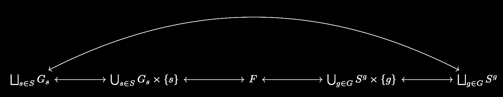 where \(F\) is the set of all formulas of the aforementioned form and all of the arrows are bijections. In particular, the bijection \(\bigsqcup_{s\in S}{G_s}\leftrightarrow\bigsqcup_{g\in G}{S^g}\) implies that
\[\sum_{s\in S}{|G_s|}=\sum_{g\in G}{|S^g|},\] and we are done. \(\square\) Burnside's lemma finds application in places where we wish to compute the number of orbits \(N\). For instance, consider the set \(S\) of \(\binom{8}{4}=70\) colorings of an octagon where four of the edges must be black and the other four must be white. Since it forms the symmetries of the octagon, the dihedral group \(D_8\) acts on this set, and we may consider orbits of this action to correspond to unique colorings. How many unique colorings are there? By Burnside's lemma, the answer is \(\frac{1}{16}\sum_{g\in D^8}{|S^g|}\). Notice by our work above, this is the same thing as \(\frac{1}{16}\sum_{s\in S}{|G^s|}\). Why do we bother using the former sum over the latter? More deeply, why did Burnside (actually, it wasn't him) care more about expressing \(N\) in terms of \(\sum_{g\in G}{|S^g|}\) rather than \(\sum_{s\in S}{|G_s|}\)? Our example hints at the answer. \(S^g\) represents the subset of colorings that remain fixed by the single symmetry \(g\). On the other hand, \(G_s\) represents the subgroup of symmetries that remain fixed by the single coloring \(s\). A little bit of thought is sufficient to see that \(S^g\) is in general a much simpler object to understand than \(G_s\). This holds in general: if the group acting on the set has a very complicated structure, it is very difficult to study the subgroup of it that fixes a single element of the set that it acts on. On the other hand, sets do not have any structure—they only have elements. By holding a group element fixed, the task becomes a matter of checking which elements in the set are fixed by that group element. This is a much easier task as it avoids the trouble of dealing with a potentially complicated group structure. In our case, this is to say that it is much easier to find the set of colorings that remain fixed under a given symmetry of the octagon than it is to find the set of symmetries that fix a given coloring of the octagon. We can push group actions even further. Let \(G\) be a group. Let \(S\) be a set, and let \(\mathrm{Perm}\ S\) denote its permutations. Note that in the category of sets, the morphisms are just functions, so \(\mathrm{Perm}\ S\) is really just the automorphism group of \(S\). In particular, it has a group structure, and there may exist a homomorphism \(\varphi\colon G\to\mathrm{Perm}\ S\). Such a homomorphism is called a permutation representation of \(G\) (with respect to \(S\)). It is not hard to see that the set of group actions of \(G\) on \(S\) has a bijective correspondence with the set of permutation representations of \(G\) with respect to \(S\). For example, let \(A\) be a group action. Then it can be checked that the map \(\varphi_A\colon G\to S_n\) which sends \(g\in G\) to the automorphism on \(S\) which is \(A\)-multiplication by \(g\) is indeed a homomorphism. Conversely, it may be checked that any permutation representation defines an action of \(G\) on \(S\). This natural correspondence gives us a natural way to identify group actions. If the permutation representation corresponding to a group action is injective, we say that the group action is faithful. Faithfulness is of course equivalent to the kernel of the corresponding permutation representation being trivial. The identity element of \(\mathrm{Perm}\ S\) is of course the identity map from \(S\) to itself. So for the kernel to be trivial, we wish left-multiplication by \(g\) to emulate the identity map on \(S\) precisely when \(g\) is the identity element of \(G\). We are now ready to prove a result that seems very deep to me at least. Cayley's Theorem: Every finite group of order \(n\) is isomorphic to a subgroup of the symmetric group \(S_n\). Proof: Let \(G\) be a finite group. Consider the group action of \(G\) on itself that maps \((g,x)\mapsto gx\). There exists a permutation representation of \(G\) with respect to itself, namely the homomorphism \(\varphi\colon G\to\mathrm{Perm}\ G\) that maps \(g\) to the automorphism on \(G\) that is left-multiplication by \(g\). Of course, the only element \(g\in G\) such that \(gx=x\) for every \(x\in G\) is the identity, so this group action is faithful. In particular, \(\varphi\) is an injective homomorphism, so \(G\) is isomorphic to \(\varphi(G)\). But of course, \(\mathrm{Perm}\ G\) is isomorphic to \(S_n\) where \(n=|G|\). \(\square\) So in an abstract sense, the symmetric groups are complicated enough that they encode every other possible finite group. This is an interesting result. However, it turns out that the idea of a group acting on itself is what really matters here, and it is that concept which is eventually used to obtain the Sylow theorems. One of the greatest advantages of the Lebesgue integral over the Riemann integral is its good behavior under limits. There are three big theorems in measure theory that demonstrate this feature of the Lebesgue integral. The first of these is the monotone convergence theorem.
Monotone Convergence Theorem: If \(\{f_n\}\) is a convergent sequence in \(L^+\) such that \(f_j\leq f_{j+1}\) for all \(j\), then \(\int{\lim_{n\to\infty}{f_n}}=\lim_{n\to\infty}{\int{f_n}}\). Proof: Suppose that the measure space we are working in is \((X,\mathscr{M},\mu)\). First, note that \(\{f_n\}\) is an increasing sequence of functions, so \(\{\int{f_n}\}\) is an increasing sequence of real numbers. Thus, \(\lim_{n\to\infty}{\int{f_n}}\) exists, at least in the extended real numbers. Put \(f=\lim_{n\to\infty}{f}\). Secondly, since \(\int{f_n}\leq\int{f}\) for all \(n\), we also have that \(\lim_{n\to\infty}{\int{f_n}}\leq\int{f}\). It remains to prove the reverse inequality. Pick a simple function \(\phi\) such that \(0\leq\phi\leq f\). Let \(\alpha\in(0,1)\) be arbitrary. Define \(E_n=\{x\in X\colon f_n(x)\geq \alpha\phi(x)\}\). Since the \(f_n\) are increasing, \(f_n(x)\geq\alpha\phi(x)\) will imply \(f_m(x)\geq\alpha\phi(x)\) for all \(m\geq n\). Hence, the \(E_n\) are an increasing sequence of sets: \(E_1\subseteq E_2\subseteq \dots\). Fix \(x\in X\). The sequence \(\{f_n(x)\}\) is an increasing sequence of real numbers converging to \(f(x)\). Hence, there exists some \(N\) such that for all \(n>N\) we have that \(0\leq f(x)-f_n(x)\leq f(x)-\alpha\phi(x)\). So for all \(n>N\) we have \(f_n(x)\geq\alpha\phi(x)\) so \(x\in E_n\). In particular, \(X=\bigcup_{n=1}^{\infty}{E_n}\). By the definitions, we have \[\int{f_n}\geq\int_{E_n}{f_n}\geq\alpha\int_{E_n}{\phi}.\] Hence, \[\lim_{n\to\infty}{\int{f_n}}\geq\alpha\lim_{n\to\infty}{\int_{E_n}{\phi}}.\] Recall that for \(E\in\mathscr{M}\), the map \(E\mapsto\int_{E}{\phi}\) is itself a measure, say \(\nu\). Since the \(E_n\) are increasing, by continuity from below on the measure \(\nu\), we have that \[\lim_{n\to\infty}{\int_{E_n}{\phi}}=\int_{\bigcup_{n=1}^{\infty}{E_n}}{\phi},\] so our inequality becomes \[\lim_{n\to\infty}{\int{f_n}}\geq\alpha\int{\phi}.\] Since this holds for \(\alpha\in(0,1)\), it will hold for \(\alpha=1\). Hence, \[\lim_{n\to\infty}{\int{f_n}}\geq\int{\phi}.\] Finally, taking the supremum over all simple functions \(\phi\leq f\), we obtain the desired inequality \[\lim_{n\to\infty}{\int{f_n}}\geq\int{f}.\] \(\square\) The definition of \(\int{f}\) requires us to consider the supremum of the set of integrals of simple functions that do not exceed \(f\), but the monotone convergence theorem tells us that we may instead compute the integral as \(\int{f}=\lim_{n\to\infty}{\int{\phi_n}}\), where \(\{\phi_n\}\) is an increasing sequence of simple functions that converges to \(f\) almost everywhere. It is a standard first result in measure theory that such sequences of simple functions exist. The monotone convergence theorem allows us to interchange integrals with limits when the limit is taken on a sequence of increasing functions. But if the dream is to be able to interchange the integral with a limit for all sequences of functions, we must prepare to be disappointed. The classic pathology is the sequence of mass functions \(f_n=\chi_{(n,n+1)}\). Of course, the sequence \(\{f_n\}\) converges pointwise to the function \(f(x)=0\), but \(\int{f_n}=1\) for all \(n\), so we clearly cannot interchange the limit and the integral in this scenario. The issue here is that even though there is convergence to a nice function, there is a non-negligible mass that preserved in every function of the sequence. A related example is given by \(f_n=n\chi_{\left(0,\frac{1}{n}\right)}\). Once again, the integral of each function in the sequence is \(1\), but the function converges pointwise to \(0\). Again, the issue is that there is a non-negligible mass that is preserved in every function of the sequence. A reasonable objection may be the following. In both examples above, the convergence is pointwise but not uniform, so perhaps the limit and integral fail to be interchangeable because the convergence is not strong enough. This is also wrong: consider \(f_n=\frac{1}{n}\chi_{(0,n)}\). In this case, \(f_n\to 0\) not just pointwise, but uniformly. Nonetheless, \(\int{f_n}=1\) for every \(n\), so the limit and integral cannot be interchanged. It turns out that the relationship between the standard modes of convergence and the limiting behavior of integrals is a subtle one which I will talk about in the future. So the failures that we have demonstrated are truly an inherent limitation of the Lebesgue integral, not a weakness of the form of convergence. Nonetheless, there is something we can say when we have no condition on the sequence of functions (not even the condition that they converge to something). Fatou's Lemma: If \(\{f_n\}\) is any sequence in \(L^+\), then \[\int{\liminf{f_n}}\leq\liminf{\int{f_n}}.\] Proof: For every \(k\geq1\) and \(j\geq k\) we have that \(\inf_{n\geq k}{f_n}\leq f_j\) and thus \(\int{\inf_{n\geq k}{f_n}}\leq\int{f_j}\). This is preserved when we take the infimum of the left: \[\int{\inf_{n\geq k}{f_n}}\leq\inf_{j\geq k}{\int{f_j}}.\] For every \(k\), let \(g_k=\inf_{n\geq k}{f_n}\) and consider the sequence of functions \(\{g_k\}\). Clearly,\(g_1\leq g_2\leq\dots\). So by the monotone convergence theorem, we have that \[\int{\liminf_{n\to\infty}{f_n}}=\int{\lim_{k\to\infty}{g_k}}=\lim_{k\to\infty}{\int{g_k}}\leq\lim_{k\to\infty}{\inf_{j\geq k}{\int{f_j}}}=\liminf_{n\to\infty}{\int{f_n}}.\] \(\square\) Fatou's lemma can be used to derive another proof of the monotone convergence theorem. Second Proof (Monotone Convergence Theorem): Recall that in the first proof, it was immediate that \(\lim_{n\to\infty}{\int{f_n}}\leq\int{f}\), so it suffices to show the reverse inequality. But this is immediate by Fatou's lemma. In particular, if a limit exists, it is equal to the limit infimum, so \(f=\liminf_{n\to\infty}{f_n}\) and \(\lim_{n\to\infty}{\int{f_n}}=\liminf_{n\to\infty}{\int{f_n}}\). \(\square\) Fatou's lemma has weak hypotheses but is a weak result. Moreover, one may ask: what about sequences in \(L^1\)? So far we have only been dealing with sequences in \(L^+\). The dominated convergence theorem is the main result that we use in practice, and is arguably one of the most important results in measure theory. Dominated Convergence Theorem: Let \(\{f_n\}\) be a convergent sequence in \(L^1\) such that there exists \(g\in L^1\) with \(|f_n|\leq g\) almost everywhere for all \(n\), then \(\lim_{n\to\infty}{f_n}\in L^1\) and \(\int{\lim_{n\to\infty}{f_n}}=\lim_{n\to\infty}{\int{f_n}}\). Proof: Let \(\lim_{n\to\infty}{f_n}=f\) almost everywhere. Some standard results show that \(f\) is measurable. Since \(|f|\leq g\in L^1\), we must have that \(f\in L^1\). Suppose that the \(f_n\) are real-valued. By the hypothesis, we have that \(g+f_n\geq0\) and \(g-f_n\geq0\) almost everywhere. Now we can compute \[\begin{split} \int{g}+\int{f}&=\int{g+f}\\ &=\int{\left(g+\lim_{n\to\infty}{f_n}\right)}\\ &=\int{\liminf_{n\to\infty}{\left(g+f_n\right)}}\\ &\leq\liminf_{n\to\infty}{\int{(g+f_n)}}\\ &=\int{g}+\liminf_{n\to\infty}{\int{f_n}}, \end{split}\] where we invoke Fatou's lemma to obtain the inequality. Similarly, \[\begin{split} \int{g}-\int{f}&=\int{g-f}\\ &=\int{\left(g-\lim_{n\to\infty}{f_n}\right)}\\ &=\int{\liminf_{n\to\infty}{\left(g-f_n\right)}}\\ &\leq\liminf_{n\to\infty}{\int{(g-f_n)}}\\ &=\int{g}-\limsup_{n\to\infty}{\int{f_n}}. \end{split}\] Rearranging the two inequalities gives us \(\liminf_{n\to\infty}{\int{f_n}}\geq\int{f}\) and \(\int{f}\geq\limsup_{n\to\infty}{\int{f_n}}\). So it follows that \[\int{f}=\lim_{n\to\infty}{\int{f_n}}.\] In general, if the \(f_n\) are not real-valued, we can break it up into the positive and negative parts of its real and imaginary parts and apply the same procedure as above to arrive at the conclusion. \(\square\) The dominated convergence theorem shows up in the proofs of many other foundational theorems of measure theory, as it accepts a mild hypothesis and permits one to interchange a limit and integral in exchange, which is a very useful operation. To get some more feel for the three big convergence theorems, we will interpret them in a special case. Consider the measure space \((\mathbb{N},\mathscr{P}(\mathbb{N}),\mu)\) where \(\mu\) is the counting measure. Let \(\{f_n\}\) be an arbitrary sequence in \(L^+\) (with respect to this measure space). What does this really mean? For each \(n\), we may construct the family of simple functions \(\{\phi_m^n\}\) as follows. First, define \[\phi_1^n=f_n(1)\chi_{f_n^{-1}(f_n(1))}.\] Define, \[A_m=\mathbb{N}\setminus\bigcup_{j=1}^{m}{f_n^{-1}(f_n(k))}.\] For \(m>1\), if \(A_m=\varnothing\), set \(\phi_m^n=\phi_{m-1}^n\). Otherwise, let \(k_m\) be the minimal element of \(A_m\) and set \[\phi_m^n=\phi_{m-1}^n+f_n(k_m)\chi_{f_n^{-1}(f_n(k_m))}.\] Observe that by construction, \(\lim_{m\to\infty}{\phi_m^n}=f_n\) everywhere, and \(m\), \(\phi_1^n\leq\phi_2^n\leq\dots\leq f_n\). So by the monotone convergence theorem, \[\int{f_n}=\lim_{m\to\infty}{\int{\phi_m^n}}=\sum_{k=1}^{\infty}{f_n(k)},\] where the sum comes from the construction of \(\phi_m^n\) and the fact that \(\mu\) is the counting measure. So we may interpret \(\int{f_n}\) as simply the sum of its values. In particular, there is a correspondence between functions in \(L^+\) with respect to our measure space and sequences of numbers in \([0,\infty]\). Let \(\{S_n\}\) be a family of such sequences, where \[S_n=s_{n,1},s_{n,2}\dots\] and let \(\{f_n\}\) be the family of functions in \(L^+\) such that \(f_n(k)=s_{n,k}\). Let \(T\) be the sequence given by \[T=t_1,t_2,\dots\] where \(t_k=\liminf_{n\to\infty}{s_{n,k}}\). Corresponding to this sequence is the function \(\liminf_{n\to\infty}{f_n}\). Hence, Fatou's lemma tells us that \[\sum_{k=1}^{\infty}{\liminf_{n\to\infty}{s_{n,k}}}\leq\liminf_{n\to\infty}\sum_{k=1}^{\infty}{s_{n,k}}.\] Now, let us further insist that the sequences \(S_n\) are such that for each \(k\), \(s_{1,k}\leq s_{2,k}\leq\dots\). Of course, for each \(k\), \(\lim_{n\to\infty}{s_{n,k}}\) is guaranteed to exist due to the compactness of \([0,\infty]\). Then by the monotone convergence theorem, \[\lim_{n\to\infty}{\sum_{k=1}^{\infty}{s_{n,k}}}=\sum_{k=1}^{\infty}{\lim_{n\to\infty}{s_{n,k}}}.\] We need some extra work to interpret the dominated convergence theorem in this context. Integrals of functions \(\mathbb{N}\to\mathbb{C}\) can still be interpreted as the infinite sum of their values by splitting up the function into the positive and negative parts of its real and imaginary parts and applying our work above on \(L^+\) functions, and using the linearity of the integral. Suppose that \(\{f_n\}\) is a sequence of functions \(\mathbb{N}\to\mathbb{C}\) in \(L^1\) such that \(f_n\to f\) almost everywhere and there is a nonnegative \(g\in L^1\) such that \(g\geq|f_n|\) almost everywhere for each \(n\). Note that the functions \(|f_n|\) are in \(L^+\), and by our previous interpretation of such functions, they correspond to sequences of numbers from \([0,\infty]\). Hence, the condition \(f_n\in L^1\) is equivalent to \[\sum_{k=1}^{\infty}{|f_n(k)|}<\infty.\] Observe that in the measure space \((\mathbb{N},\mathscr{P}(\mathbb{N}),\mu)\), the only null set is the empty set. Hence, convergence almost everywhere is equivalent to convergence everywhere in this context. In particular, for each \(k\), \(f(k)=\lim_{n\to\infty}{f_n(k)}\). Moreover, notice that \(g\) is in \(L^+\), so \[\sum_{k=1}^{\infty}{|f_n(k)|}\leq\sum_{k=1}^{\infty}{g(k)}<\infty.\] So the interpretation is the following. Let \(\{S_n\}\) be a family of sequences of complex numbers \[S_n=s_{n,1},s_{n,2},\dots,\] such that for each \(k\), \(\lim_{n\to\infty}{s_{n,k}}\) exists, and there exists a sequence of nonnegative real numbers \(s_1,s_2,\dots\) with \[\sum_{k=1}^{\infty}{|s_{n,k}|}\leq\sum_{k=1}^{\infty}{s_k}<\infty,\] for each \(n\). By the dominated convergence theorem, \[\sum_{k=1}^{\infty}{\lim_{n\to\infty}{s_{n,k}}}=\lim_{n\to\infty}{\sum_{k=1}^{\infty}{s_{n,k}}},\] and moreover, \[\sum_{k=1}^{\infty}{\lim_{n\to\infty}{|s_{n,k}|}}<\infty.\] |
Categories
All
Archives
July 2023
|
 RSS Feed
